1Introduction
Magnetization Transfer (MT) imaging encompasses a family of MRI techniques that exploit the interactions between different proton populations in biological tissues to generate unique contrast mechanisms. At its core, MT imaging examines the exchange of magnetization between highly mobile water protons (the “free pool”) and protons associated with macromolecules and semi-solid structures (the “restricted pool”). The restricted pool protons have ultrashort transverse relaxation times (T2 ~ 10-50 μs), making them undetectable with conventional MRI techniques. This ultrashort T2 leads to substantial frequency broadening of the restricted pool’s absorption lineshape, which MT techniques leverage by applying off-resonance radiofrequency pulses that selectively saturate macromolecular protons while minimally affecting the free water pool Wolff & Balaban, 1989Henkelman et al., 1993.
The pervasive nature of MT effects means that virtually all MRI sequences are impacted by MT interactions. Even on-resonance pulses can pump the restricted pool, which subsequently exchanges magnetization with the water pool, particularly for sequences that use large flip angles such as inversion pulses and spin-echo trains. Off-resonance effects are especially pronounced in multi-slice acquisitions, where RF pulses intended for neighboring slices can inadvertently saturate macromolecular protons in the slice of interest Santyr, 1993. These MT effects can significantly bias quantitative MRI measurements, contributing substantially to the challenges of standardizing quantitative MRI across different platforms and protocols. Ignoring MT effects has been shown to bias T1 mapping Assländer & Flassbeck, 2025Assländer, 2025 and T2 mapping, where the extensive use of radiofrequency pulses in multi-echo sequences can lead to underestimation of relaxation times. By deliberately manipulating these exchange processes through specialized RF preparation pulses, MT techniques can generate contrast that reflects macromolecular density and organization Sled, 2018, providing valuable insights into tissue microstructure that complement conventional relaxation-based contrasts.
By deliberately manipulating these exchange processes through specialized RF preparation pulses, MT techniques can generate contrast that reflects macromolecular density and organization Sled, 2018. This capability has enabled important applications across clinical and research domains, particularly for assessing myelin content in neurological disorders such as multiple sclerosis Schmierer et al., 2004Schmierer et al., 2007, and has also shown utility in studying Alzheimer’s disease Fornari et al., 2012 and psychiatric disorders Chen et al., 2015.
This chapter explores three principal methodologies for magnetization transfer imaging, each offering different levels of quantitative rigor and practical implementation. Quantitative Magnetization Transfer (qMT) represents the most comprehensive approach, employing multi-parameter fitting of the Bloch-McConnell equations to extract fundamental tissue properties such as pool size ratio, exchange rates, and relaxation times Sled & Pike, 2001Sled, 2018. While providing the most detailed characterization of tissue microstructure, qMT requires extensive acquisition protocols and complex fitting procedures, making it challenging for routine clinical use. In contrast, Magnetization Transfer Ratio (MTR) offers a simplified, semi-quantitative approach that calculates the normalized signal difference between images acquired with and without MT preparation Wolff & Balaban, 1989. Despite its widespread clinical adoption, particularly in multiple sclerosis research, MTR suffers from dependencies on sequence parameters and tissue relaxation properties that limit its quantitative accuracy.
More recently, Magnetization Transfer Saturation (MTsat) has emerged as an intermediate approach that combines the practicality of MTR with improved quantitative characteristics Helms et al., 2008. By incorporating additional measurements and analytical corrections, MTsat provides better separation of MT effects from confounding factors like tissue T1 variations, while maintaining clinically feasible acquisition times. Throughout this chapter, we will examine the theoretical foundations, practical implementations, and relative strengths of each MT imaging approach, providing readers with comprehensive understanding of how these techniques can be applied to study tissue microstructure across various research and clinical contexts.
2Quantitative Magnetization Transfer
Magnetization Transfer (MT) has been extensively applied to study macromolecular biological tissue composition. The imaging contrast resides in the magnetization transfer between free-water protons and macromolecular proton compartments, through chemical exchange and dipolar interactions. In the two-pool tissue model, highly mobile protons are associated with the free-water pool while protons found in semisolid macromolecular sites are defined as the restricted pool Sled, 2018. A simple method for visualizing MT effects includes acquiring two images with and without an off-resonance MT pulse to calculate the MT ratio (MTR), which is the normalized difference of these two images Wolff & Balaban, 1989. Despite its proven usefulness to study multiple sclerosis Zheng et al., 2018, Alzheimer’s disease Fornari et al., 2012 and psychiatric disorders Chen et al., 2015, the MTR is a semi-quantitative metric that depends critically on the imaging sequence parameters Seiberlich et al., 2020. Another semi-quantitative approach is the estimation of MT saturation (MTsat) by fitting the MT signal obtained from an MT-weighted (MTw), a proton density (PD) weighted and T1-weighted (T1w) contrast Helms et al., 2008. Quantitative MT (qMT) consists of fitting multiple images to a mathematical model to extract tissue-specific parameters related to physical quantities, such as pool sizes, magnetization exchange rates between pools, and T1, T2 relaxation times of each pool. Compared to semi-quantitative approaches (MTR, MTsat), qMT has long acquisition protocols and sometimes needs additional measurements (eg. B0, B1, T1), and the complex models required to fit the quantitative maps makes it a challenging imaging technique.
In 2015, our lab published qMTLab Cabana et al., 2015, an open-source software project seeking to unify three qMT methods in the same interface: qMT using spoiled gradient echo (qMT-SPGR), qMT using balanced steady-state free precession (qMT-bSSFP), and qMT using selective inversion recovery with fast spin echo (qMT-SIRFSE). qMTLab allowed users to simulate, evaluate, fit, and visualize qMT data with the possibility to share qMT protocols between researchers, allowing them to compare the performance of their methods Cabana et al., 2015. Since then, we have extended the project and renamed it to qMRLab, Karakuzu et al., 2020, which in addition to qMT now provides over 20 quantitative techniques under one umbrella, such as relaxation and diffusion models, quantitative susceptibility mapping, B0 and B1 mapping. In addition, we created interactive tutorials (see the T1 mapping chapters using the inversion recovery, variable flip angle, and MP2RAGE techniques) and blog posts for several qMRI techniques that were published under a creative commons license made it into a quantitative MRI book published by Elsevier Seiberlich et al., 2020. This blog post is a continuation of our qMRLab outreach initiative, where we will focus on qMT and the tools we provide in qMRLab for this class of techniques.
This section is an introduction to qMT (with a focus on qMT-SPGR), where we will cover signal modelling and data fitting.
Signal Modelling
The magnetization transfer in a two-pool model is modelled by a set of coupled differential equations Sled & Pike, 2000:
where the magnetization at time t is given by and and are the transverse magnetization for the free pool in the x and 𝑦 direction, respectively. The longitudinal magnetization for the free and restricted pool is denoted by and . Due to the very short T2 of the restricted pool (on the order of microseconds), the transverse magnetization of this pool is not explicitly modelled.
The constants kf and kr represent the exchange rate of the longitudinal magnetization from the free pool to the restricted pool (kf) and from the restricted to the free pool (kr). The ratio of these quantities is constrained by the size of the restricted to the free-water pool, expressed as . This ratio is called the pool size ratio F defined as . The precessional frequency is a measure of the power of the off-resonance radiofrequency pulse and ∆ is a frequency offset at which the magnetic B1+ field is applied. As shown in Figure 6.1, an on-resonance (∆ = 0) radiofrequency pulse is also part of the pulse sequence and is applied after the MT pulse. The relaxation time constants for the free and restricted pools are denoted by T1,f and T1,r for the longitudinal magnetization, and T2,f and T2,r for the transverse magnetization. Finally, 𝑊 is the saturation rate of the restricted pool, which is a function of the absorption lineshape 𝐺 that depends on the frequency offset and the transverse relaxation of the restricted pool (Figure 6.2).
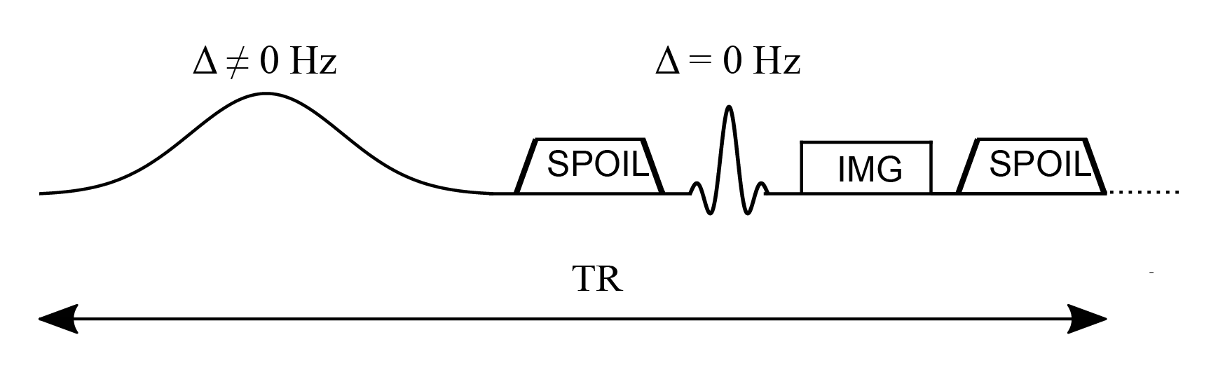
Figure 6.1:Simplified pulse sequence diagram of a magnetization transfer spoiled gradient (MT-SPGR) experiment with an MT pulse followed by a spoiler gradient to destroy any transverse magnetization before the application of the on-resonance excitation pulse.
The absorption lineshape of the restricted pool that best characterizes the proton system depends on the environment. For simple systems such as agar gel phantoms, the Gaussian lineshape describes magnetization transfer effects well Henkelman et al., 1993, while for more complicated and biologically relevant models, the super-Lorentzian lineshape is the best choice Morrison et al., 1995.
Figure 6.2:Gaussian, Lorentzian and super-Lorentzian absorption lineshapes plotted as a function of the frequency offset ∆ and T2,r.
In a standard qMT experiment, multiple measurements are required where the off-resonance radiofrequency pulse angle (MT angle) and offset frequency are changed for each measurement, and at least one measurement is acquired in the absence of an MT pulse. The acquired signal plotted as a function of the offset frequency is known as the “Z-spectrum”, and Figure 6.3 shows the Z-spectrum simulated using different absorption lineshapes. The off-resonance MT pulse is modelled either as a continuous wave or as a pulsed irradiation scheme. In a continuous wave irradiation mode, long off-resonance pulses of constant saturation and fixed frequency offset are applied to generate well-defined MT states in the two pools Henkelman et al., 2001. For more practical implementations, pulsed off-resonance irradiations are used with a spoiled gradient echo sequence (SPGR) to generate MT-weighted images at different saturation rates and frequency offsets Sled & Pike, 2000. In the qMT-SPGR sequence shown in Figure 6.1, the MT preparation pulse is applied, followed by a spoiler gradient to eliminate any residual transverse magnetization produced by the long MT pulses, and to destroy the MR signal from previous measurements. A signal equation for this type of pulsed MT experiment can be derived by approximating the pulse sequence to a series of stages described by a continuous wave off-resonance irradiation period, followed by free precession, and instant saturation of the free-water pool Cabana et al., 2015Sled & Pike, 2000Sled & Pike, 2001. This pulse sequence decomposition allows for analytically solving the Bloch-McConnell equations at a steady-state, but it is also possible to numerically solve the Bloch equations to perform simulations that provide a more realistic approximation when the system has not been driven to a steady-state. A comparison between the Bloch simulations and the analytical solution is shown in Figure 6.4 for different numbers of preparation MT pulses. As can be seen, different frequency offsets and MT flip angles require different numbers of repetition times to reach the steady-state, which is of paramount importance since the analytical solution used for parameter estimation is derived assuming the steady-state. In terms of data acquisition optimization, the k-space periphery is sampled during the preparation pulses whereas the center of k-space, that contains the overall image contrast, is acquired once the steady-state is achieved.
Figure 6.3:Z-spectrum simulated using different absorption lineshapes (Gaussian, Lorentzian, and super-Lorentzian).
Figure 6.4:Z-spectrum simulated using Bloch simulations (dashed lines) for a number of MT pulses ranging from 1 to 600. Bloch simulations are compared with the Z-spectrum obtained from the analytical solution (solid lines).
Data Fitting
In qMT imaging, the biophysical model relates the parameters observed in the two-pool tissue model to physical quantities such as the fractional size of the pools, relaxation times and magnetization exchange rates of the free and restricted pool Sled & Pike, 2001Sled, 2018. However, qMT experiments usually consist of long acquisition imaging protocols accompanied by complex data fitting. To this end, some software solutions have been proposed Karakuzu et al., 2020Tabelow et al., 2019C Wood, 2018. qMRLab is an open-source project for quantitative MR analysis that is an extension of qMTLab, a software for data simulation and analysis of three MT models: qMT-SPGR, qMT-bSSFP and qMT-SIRFSE. In addition to the quantitative MT methods, qMRLab also contains semi-quantitative MT models including the magnetization transfer ratio (MTR) and magnetization transfer saturation (MTsat).
The qMT-SPGR method in qMRLab contains three fitting models: Sled and Pike, Ramani, and Yarnykh and Yuan Sled & Pike, 2001Ramani et al., 2002Yarnykh, 2002. For the Sled and Pike model, the saturation fraction effect of the MT pulse on the free pool is pre-computed to accelerate the processing times. The MT effect of the pulse is approximated as an instantaneous fractional saturation of the longitudinal magnetization of the free pool, assuming the absence of chemical exchange processes Pike, 1996Sled & Pike, 2001. To fit the model, additional parameters related to the pulse sequence are required, namely timing parameters, the absorption lineshape, and the characteristics of the MT pulse, such as the shape and the bandwidth or the time-bandwidth product. In Figure 6.5, the qMT-SPGR method is used to show a single voxel curve simulation for the same MT data fitted by three different models. The fitted parameters were the pool size ratio F, the magnetization transfer rate from the restricted to the free-water pool (kr), and the transverse relaxation time of the free-water (T2,f) and restricted (T2,r) pool.
Figure 6.5:Sled and Pike, Ramani, and Yarnykh and Yuan models to fit the MT data from a qMT-SPGR experiment.
In addition to acquiring the MT data, three more quantitative measurements are typically required for model correction purposes. The magnetic field B0 inhomogeneity affects the actual off-resonance frequency experienced by the tissue at each voxel. In MT, B0 maps are computed to correct for off-resonance frequency values of the MT pulse in the presence of magnetic field non-uniformity. Radiofrequency field B1 inhomogeneity is another source of inaccuracies that depend on the operating frequency of the scanner, the pulse sequence, and the shape and electrical properties of the sample Sled & Pike, 1998. Therefore, B1 maps are typically needed to correct the radiofrequency amplitude variations that affect the nominal values of the MT pulse flip angle and the excitation flip angle Boudreau et al., 2018. Longitudinal relaxation T1 values vary naturally in biological tissue, but the choice of the T1 mapping method, has also been shown to influence the variability of T1 measurements Stikov et al., 2015. In the context of a qMT experiment, T1 maps are acquired with an independent measurement of the apparent relaxation time T1 (T1, meas). The T1 map is related to the relaxation rate of the free pool (R1,f) as described by Eq. 6.6, expressed in terms of 𝐹, kf, R1,meas and R1,r, where the relaxation rate of the restricted pool is arbitrarily set to 1 s-1 because it is insensitive to this kind of MT experiments Sled & Pike, 2001. Multiple qMRI maps with a range of B0 and B1 inaccuracies, as well as T1 maps with a variety of relaxation times, have been simulated to show the effect of the quality of these input maps on the qMT fitted parameters as shown in Figure 6.6.
Figure 6.6:Errors (%) in fitted parameters when input maps of different quality are used. A B1 map of 0.9 means that the input has a 10% lower value than expected. The fitted parameters include the pool size ratio, F, the magnetization exchange rate, kf, the free pool T2,f, and the restricted pool T2,r. The errors were simulated for B0, B1 and T1 maps of different quality.
As described above in Figure 6.6, inaccurate MT pulse flip angles and excitation flip angles affect the fitted MT parameters, and there is an additional error source related to the T1 mapping measurement. As shown in Boudreau et al., 2018, using specific acquisitions protocols, T1 values can be affected by B1 field non-uniformities, such as the variable flip angle method, while the inversion recovery method is insensitive to these field inhomogeneities Stikov et al., 2015.
Figure 6.7 displays an example human dataset with the input qMRI maps used to fit the qMT parameters F, kf, T2,f, T2,r.
Figure 6.7:Example magnetization transfer spoiled gradient dataset showing qMRI maps used to fit the MT data (top), and the fitted parameters F, kf, T2,f, T2,r (bottom).
Summary
In summary, the Bloch-McConnell equations, an analytical solution to the steady-state signal can be derived and fitted with one of the existing models that make different approximations to fit the qMT data for a different set of parameters. The Sled and Pike model Sled & Pike, 2001 constrains the solution space by computing complementary T1 maps, whose acquisition method influences the B1 sensitivity of the fitted parameters Boudreau et al., 2018. This fitting model can be implemented with a continuous or a rectangular wave irradiation of the restricted pool Cabana et al., 2015. Ramani’s fitting model is an alternative approach that assumes a continuous wave irradiation scheme with the MT pulse on both free and restricted pools Ramani et al., 2002. Another fitting model was proposed by Yarnykh Yarnykh, 2002 where an analytical solution to describe the magnetization is found when the direct saturation of the free pool is neglected.
In future blog posts, we will explore other MT methods, such as MTR Wolff & Balaban, 1989, MTsat Helms et al., 2008 and qMT-bSSFP Bieri & Scheffler, 2007Gloor et al., 2008. Additionally, we will also be looking at the effects of RF field inhomogeneity on the generated magnetization transfer maps.
3Magnetization Transfer Ratio
Conventional MRI techniques, such as those used for clinical diagnosis, can only directly measure hydrogen bonded to water molecules. Thus, a non-negligible proportion of body mass is not visible with clinical MRIs, such as non-hydrogen atoms (different resonance frequencies) and hydrogen atoms bonded to large molecules which restricts the motion of the atoms (rapid signal decay, T2 ~ μs). The latter, called macromolecules, play an important role in the physiology of the body; for example, myelin in the white matter of the brain plays an important role in signal transmission, and is composed largely of macromolecules (lipids and proteins). Although the images acquired by clinical MRI machines can only be generated from signal from mobile hydrogen, these hydrogen atoms interact with nearby molecules and atoms via the electromagnetic fields they mutually generate. In the 70s and 80s, a cross-relaxation mechanism was discovered that sensitizes mobile protons to nearby targeted semi-solid molecules, such as myelin Edzes & Samulski, 1977Edzes & Samulski, 1978Wolff & Balaban, 1989. With proper experimental design, a higher density of nearby macromolecules in the tissue results in a lower MRI signal. This class of MRI techniques is known as magnetization transfer (MT) imaging.
In the preceding chapter, we delved into the quantitative aspects of magnetization transfer (qMT) imaging, exploring the Bloch-McConnell model, signal modeling, and fitting techniques using qMRLab. Now, we shift our focus to the more accessible and widely used application of MT: magnetization transfer ratio (MTR). Although less quantitative than qMT, MTR is easier to set up and implement, making it popular choices in the MRI community interested in quantifying myelin loss.
In the simplest and most used MT imaging method, only two images are acquired (one with MT preparation, and one without), and a normalized difference between the two images is calculated. This quantity is known as the magnetization transfer ratio (MTR), and has been used extensively to infer information on myelin diseases and disorders, such as multiple sclerosis (MS). The proportional relationship between MTR and myelin density has been established using post-mortem immunohistological studies in humans Schmierer et al., 2004Schmierer et al., 2007 and animals Merkler et al., 2005Zaaraoui et al., 2008. MTR has also already been used in clinical drug trials for MS Maguire et al., 2013Brown et al., 2016. Its widespread use is due to the fact that most scanners are equipped with the necessary software so that it can be added to an imaging protocol with the click of a button, and it is also a very quick measurement with a short acquisition time.
As summarized in the previous chapter, MR physicists have also developed other MT-related techniques that aim to extract quantitative physical information of tissues, using the mathematical models that describe the MT process. This sub-field is called quantitative MT, and the tissue properties that are typically measured are: the pool-size ratio F (density of the macromolecular content’s (restricted pool) equilibrium magnetization divided by the the same value for the liquid content (free pool)), the exchange rate R, the longitudinal relaxation of the free pool T1,f, and the transverse relaxation of both the free and restricted pools (T2,f and T2,r). In contrast to MTR, quantitative MT techniques are not as widely used because of the long image acquisition times required that impedes clinical use. qMT also requires additional calibration measurements (B0, B1+, and T1), which can be challenging to measure accurately and thus contribute to additional propagation of errors to the measured qMT parameters Boudreau et al., 2018Boudreau & Pike, 2018. Despite these challenges, a lot of research focuses on developing and using qMT techniques in smaller studies, because the measured qMT parameters are desensitized to effects that can bias MTR measurements (eg T1, B1+). Another semi-quantitative MT technique that was recently developed is the MT saturation (MTsat) technique, which is the focus of another section of this book.
MTR in theory
The full mathematical description of the magnetization transfer two-pool exchange model was explained in the qMT section. Although it’s these same equations that explain the signal differences between the two images acquired used to calculate MTR, in this section we’ll present a more conceptual explanation of the MT exchange process.
In its most basic form, MT is modeled as an exchange process between two “pools” of protons, those from “mobile” protons (eg, hydrogen in liquid water) named the “free” pool (those that are directly measured with conventional MRI), and those from “restricted” protons (i.e. macromolecules) named the “restricted” pool (these cannot be measured directly with conventional MRI). Macromolecular hydrogen cannot be measured directly because the restricted movement creates a more static local electromagnetic environment that doesn’t average out, and this results in a transverse relaxation T2,r (signal decay) that is too short to provide measurable signal (T2,r ~ μs << feasible TE). Another consequence of this short signal decay time is a broadening of the absorption lineshape in the frequency domain (eg. the range of “resonant” frequencies of that pool of protons). This is a known property of the Fourier Transform, and the phenomenon is isomorphic to the quantum mechanics uncertainty principle; as Δx⋅Δp ≥ constant in quantum mechanics means that if Δx increases Δp will decrease, we observe a similar relationship approximated to T2⋅FWHM (full width at half maximum) of the frequencies = constant such that if T2 decreases, the FWHM of the frequencies will increase. If T2 is very very short (such as the case for macromolecules), the range of resonant frequencies will be very wide. MT leverages this property by selectively exciting restricted protons far from the mobile proton resonance frequency (applying a pulse off-resonance), but where the energy will be absorbed by some of the protons in the restricted pool. This is the initial preparation of the MT experiment that triggers the conditions needed for cross-relaxation between the unobservable molecules (restricted pool) and observable protons (free pool).
Conventionally, the two-pool exchange model is explained conceptually as a process of magnetization exchange, which is also how it’s described mathematically using the Bloch-McConnel equations. However, this conceptual model can be challenging to understand, particularly for people with physics backgrounds, because unlike energy and momentum, the total magnetization in a voxel is not a conserved physical property. This can be seen simply by observing the evolution of the total magnetization vector after an excitation pulse; the total magnetization vector is (mostly) conserved during the RF pulse, but then decays quickly to near 0 due to T2 relaxation, and takes a long time to grow back to M0 from T1 relaxation. The vector is not constant. So, if magnetization is not a conserved property, how do we know if and how much of it is being exchanged?
As explained in more detail in Appendix A, an MT experiment involves the conservation and transfer of energy between spin populations. The off-resonance RF pulse introduces extra energy into the restricted pool of protons, and the relaxation back to thermal equilibrium occurs through spin-lattice relaxation, where the “lattice” includes nearby free-pool protons. This energy exchange results in a reduction of net magnetization in the free pool and a corresponding decrease in observable MR signal. This process underlies the contrast observed in MT imaging, which reflects differences in tissue microstructure and composition.
Now that we have a better grasp of the magnetization exchange process, we can see how this applies for MTR. In MTR, we acquire one image with MT saturation (low signal where there is high macromolecular density), and one image without MT saturation (higher relative signal where there are macromolecules). The MTR signal is then simply calculated as a normalized difference in percentage, that is:
What does this calculated MTR value mean? MTR is the reduction in the steady-state signal resulting from an MT-sensitizing pulse and the ensuing MT exchange that occurs. The higher the density of macromolecular content there is, the more reduction in MT-weighted signal will occur, resulting in a higher MTR value. Typically, MTR values in healthy white matter are higher than in grey matter, and MTR values where there is myelin loss are smaller relative to healthy tissue.
MTR in practice
Typically, MTR imaging protocols are implemented on the scanner by adding a relatively long (~5-10 ms) high amplitude off-resonance (~2kHz) preparation RF pulse prior to each TR of an existing imaging sequence. In the early days of MT, the MT pulse was a very long pulse (~10 seconds) prior to one imaging readout of saturation-recovery sequences, but this results in impractically long acquisition times and is very SAR (Specific Absorption Rate) prohibitive. Alternative approaches were explored (eg. 1-2-1 pulses), however now most MT-weighted sequences are done using steady-state sequences (eg SPGR) with a shorter preparation pulse (~10 milliseconds). Figure 6.8 illustrated this using a spoiled-gradient recalled echo (SPGR) sequence, with a Gaussian-shaped MT preparation pulse prior to the excitation pulse.

Figure 6.8 :Simplified pulse sequence diagram of an MTR imaging sequence. An off-resonance and high powered MT-preparation pulse is followed by a spoiler gradient to destroy any transverse magnetization prior the application of the imaging sequence, in this case a spoiled gradient recalled echo (SPGR).
Each MRI vendor optimizes their MT-weighted protocol parameters (eg MT shape, duration, frequency, and amplitude), and few of these details are typically shared with the end-user. Table 6.2 shares protocol parameters used by different MRI manufacturers as reported by two publications.
Table 6.2 :Literature MTR protocol parameters (sources: Brown et al., 2013Karakuzu et al., 2022)
| Brown 2013 | Karakuzu 2022 | |||
|---|---|---|---|---|
| Siemens | Philips | GE | Siemens | |
| FA (deg) | 15 | 15 | 6 | 6 |
| TR (ms) | 30 | 47 | 32 | 32 |
| TE (ms) | 11 | 8 | 4 | 4 |
| Offset (Hz) | 1500 | 1100 | 1200 | 1200 |
| MT pulse shape | Gaussian | Sinc-Gaussian | Fermi | Gaussian |
| MT pulse length (ms) | 7.68 | 15 | 8 | 10 |
| MT pulse angle (deg) | 500 | 620 | 540 | 540 |
These differences in protocol parameters can result in MTR values that vary greatly between vendors and sites, meaning that MTR can be challenging to compare unless great care in details are taken. Figure 6.9 shows MTR simulations using the fundamental qMT parameters for four different tissues (Table 6.3 ; healthy cortical grey matter, healthy white matter, NAWM, early white matter multiple sclerosis lesion, late white matter multiple sclerosis lesion) using the four MT-weighted SPGR protocols from Table 6.2 .
Table 6.3 :Quantitative MT parameters in healthy and diseased human tissue reported for a study at 1.5 T Sled & Pike, 2001.
| Healthy cortical GM | Healthy WM | NAWM | Early WM MS lesion | Late WM MS lesion | |
|---|---|---|---|---|---|
| F | 0.072 ± 0.013 | 0.161 ± 0.025 | 0.15 ± 0.02 | 0.12 ± 0.02 | 0.094 ± 0.015 |
| kf | 2.4 ± 0.013 | 4.3 ± 1.0 | 4.9 ± 1.3 | 3.6 ± 0.8 | 2.7 ± 0.7 |
| R1,f (s-1) | 0.93 ± 0.2 | 1.8 ± 0.3 | 1.78 ± 0.4 | 1.52 ± 0.2 | 1.26 ± 0.3 |
| R1,r (s-1) | 1 | 1 | 1 | 1 | 1 |
| T2,f (ms) | 56 ± 8 | 37 ± 8 | 38 ± 7 | 43 ± 6 | 52 ± 9 |
| T2,r (μs) | 11.1 ± 8 | 12.3 ± 1.6 | 11.4 ± 1.4 | 10.3 ± 1.1 | 10.9 ± 1.4 |
Figure 6.9:MTR values calculated from fundamental qMT tissue parameters for four different MTR imaging protocols.
As demonstrated in the above simulations, one MTR value could have the same value for healthy tissue on one scanner as diseased tissue would have on another scanner. So for the most part, MTR is best used / compared within vendors at the very least, though some normalization techniques have been developed.
In addition to being very sensitive to protocol implementations, MTR values are also sensitive to other tissue properties. As seen in the qMT blog post, the parameter most closely related to macromolecular content is the pool-size ratio F. But, if some disease / symptom impacts T1 independently of underlying macromolecular content, MTR will also change. That is to say, MTR is sensitive to tissue’s T1 value independently of the macromolecular content metric F, as shown in Figure 6.10.
Figure 6.10:MTR value for (protocol?) and (tissue?) changes as a function of the underlying T1 value (T1,obsobs or T1,f?).
In addition to being sensitive to tissue properties, MTR is also sensitive to system properties such as B1 (via MT pulse amplitude) and B0 (via off-resonance frequency). In particular, B1 can vary up to 30% the nominal value at 3T, and without correction this can introduce substantial errors. Figure 6.11 illustrates how MTR can vary with different B1 values.
Figure 6.11:MTR value for (protocol?) and (tissue?) changes as a function of the underlying B1 value (T1,obsobs or T1,f?).
Lastly, MTR is sensitive to protocol adjustments, which could be done by a scanner operator to accommodate issues during an imaging session. Figure 6.12 demonstrates how MTR varies with TR adjustments.
Figure 6.12:MTR value for (protocol?) and (tissue?) changes as a function protocols TR value.
Parting thoughts
To sum up, our exploration of Magnetization Transfer Ratio (MTR) has highlighted its widespread utility within the field of MRI, in particular for myelin quantification applications. However, it’s essential to emphasize that MTR, while immensely valuable, is not a truly quantitative metric. This point underscores the need for caution when comparing MTR values or conducting longitudinal studies, as various factors, including scanner upgrades (both in hardware and software), can potentially result in variations in MTR values for the same subject or samples.
In our next section, we’ll shift our focus to MTsat, which is a promising semi-quantitative metric that rivals MTR for its ease of use and rapid acquisition times. MTsat aims to address some of the challenges associated with MTR, while still offering robust sensitivity to macromolecular content.
4Magnetization Transfer Saturation
Magnetization Transfer Saturation (MTsat) is a semi-quantitative MRI technique that offers unique insights into tissue microstructure. Built upon the spoiled gradient-recalled echo (SPGR) sequence, the MTsat protocol acquires images with and without an MT-preparation off-resonance pulse to acquire different contrast that varies with macromolecular density and T1.
The foundation of MTsat lies in a 2008 model by Helms and colleagues Helms et al., 2008, which treats the off-resonance pulse as a second excitation pulse, allowing us to model the effects of MT analytically without the need of the complex Bloch-McConnel equations. Following some reasonable approximations and the acquisition of three distinct MRI images, this model allows for analytical computation of a parameter that models the % reduction in free-pool longitudinal magnetization due to a single off-resonance pulse, MTsat.
This introduction provides a glimpse into the theoretical basis of MTsat, its practical applications, and sensitivity to variables like tissue T1 and B1. By exploring the unique properties and potential of MTsat, we hope to give readers a better understanding of the advantages and limitations of this MRI technique in both research and clinical practice, as well as give a deeper conceptual understanding of what the MTsat value means.
MTsat, like MTR and many flavours of quantitative MT, is based on spoiled gradient recalled echo (SPGR) images Haase et al., 1986Sekihara, 1987Hargreaves, 2012 preceded by an off-resonance RF pulse to provide magnetization transfer contrast Wolff & Balaban, 1989Henkelman et al., 1993Sled & Pike, 2000Sled, 2018. Figure 6.14 presents a simplified diagram of this MT-prepared SPGR pulse sequence (imaging gradients are not shown). A standard SPGR sequence (low flip angle [~5-10°], short TR [~10-30ms], and a strong spoiler gradient) are preceded by a long (~10 ms) off-resonance (~1-5 kHz) pulse with a strong peak amplitude (the total pulse has an equivalent on-resonance flip angle of 200°-700°). A smooth shape (e.g. Gaussian or Fermi) is typically used for the off-resonance pulse in order to have a single off-resonance frequency (from Fourier analysis). A strong spoiler gradient is also added between the off-resonance MT-preparation pulse and the on-resonance excitation pulse in order to destroy residual transverse magnetization that may have been created by the off-resonance pulse. Images acquired without MT saturation are acquired using the same timing as this sequence, but with the off-resonance RF pulse either completely off or using a very large off-resonance frequency (e.g. ~30+ kHz).
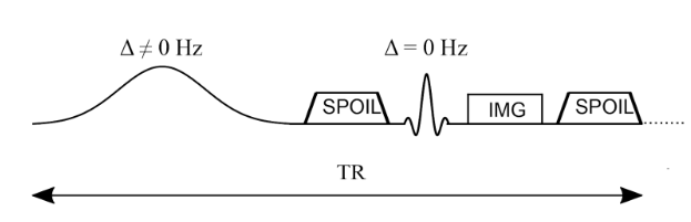
Figure 6.14:Simplified pulse sequence diagram of an MTR imaging sequence. An off-resonance and high powered MT-preparation pulse is followed by a spoiler gradient to destroy any transverse magnetization prior the application of the imaging sequence, in this case a spoiled gradient recalled echo (SPGR).
In the initial MTsat paper Helms et al., 2008Helms et al., 2010, the main innovation stems from a new model of the MT-weighted SPGR sequence shown in Figure 6.14. There, Helms et al., 2008 proposed to interpret the effects of the MT-preparation pulse as a second excitation RF pulse of an unknown flip angle. That is to say, they modeled the reduction of the longitudinal magnetization of the free pool due to the MT pulse to be the same reduction caused by the flip angle rotation of a second instantaneous excitation RF pulse. Figure 6.15 presents the Helms model, where to be consistent with the convention presented in mathematical derivations in Helms et al., 2008Helms et al., 2010, the order of the pulses are switched such that the readout excitation pulse comes first (), and the excitation pulse modelling the effects of the MT pulse comes second (). Note that, after a steady-state is reached, this order would not not impact the signal value during image readout.
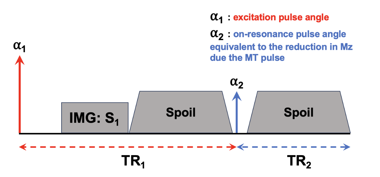
Figure 6.15 :Pulse sequence model used in MTSat to approximate the effects occurring in the actual MT-weighted sequence (Figure 6.14), but as a dual-excitation sequence. Note that the defined TR is shifted so that the beginning of the TR occurs at the excitation pulse, instead of the MT pulse as per Figure 6.14, which once a steady-state is established won’t impact the calculations.
Theory
As has been derived in many introductory MRI physics textbooks, the steady-state signal equation for a standard SPGR pulse sequence (that is, one excitation flip angle per entire TR) has been shown to be:
where A is some proportionality constant (e.g. gyromagnetic ratio, density, coil sensitivity, etc), ɑ is the excitation flip angle, R1 = 1/T1 (assuming a monoexponential longitudinal relaxation curve), and TR is the repetition time. Similarly, an analytical equation for the steady-state signal of a dual-excitation SPGR experiment (Figure 6.15 ) can be derived, and Helms et al., 2008 demonstrated it to be:
where is the imaging excitation flip angle, is the excitation flip angle representing the MT saturation pulse, TR1 is the time between to , TR2 is the time between and the following , and TR = TR1 + TR2.
Eq. 6.9 has three unknowns: A, R1, and . Of these three, is expected to be the most sensitive to macromolecular density via the MT effect, and as such is the parameter that we’d like to calculate or fit using this dual-excitation SPGR model for the MT-prepared SPGR pulse sequence. Although there would be some ways to acquire additional measurements (three unknowns, so at a minimum three measurements are needed) and apply a nonlinear fit to Eq. 6.9 to extract , this method has a long numerical processing time. To shorten the calculation of the parameter maps, Helms et al., 2008Helms et al., 2010 (Helms et al. 2008, 2010) proposed some reasonable assumptions that can be made to simplify Eq. 6.9. The first proposed assumption is that R1TR << 1, which is true when using typical MT-weighted SPGR protocol parameters (TR ~ 0.01-0.05 s) and in the brain at clinical field strengths (T1 ~ 1 s, thus R1 ~ 1 s-1). The same approximation applies to TR1 and TR2, which are shorter than TR. This leads to the removal of all exponential functions in Eq. 6.9, as via the Taylor expansion of the exponential function, exp(x) ~ 1 + x when abs(x) << 1, and the removal of another term via R1TR1R1TR2 ~ 0 when R1TR1 and R1TR2 are both << 1. The simplifications result in
The second approximation is that is small (less than 30 degrees), which is to say that the MT saturation is relatively small. This is expected to be true for the tissue properties of the brain (mostly, myelin), but care must be taken with the planned MT pulse parameters as the MT saturation increases with smaller offset frequency and high peak pulse amplitude. Later, we’ll calculate if this is a reasonable assumption for the calculated . This assumption is integrated into Eq. 6.9 via the Taylor series expansion of the , where for small x (this relationship is true for x < 30 degrees or 0.5 radians). Introducing this approximation in [3] and with the additional simplifications R1TR ~ 0 (from the assumptions above), this results in
Note how the signal no longer has a dependency on the individual TR1 and TR2 values, but only on the full TR. The final approximation is isomorphic to the previous one, but for the imaging excitation RF pulse, that is to say, that is small (less than 30 degrees). This is a controllable approximation, as it is a controllable protocol parameter at the scanner. From this assumption, and (from the Taylor series expansion), so introducing both of these into Eq. 6.11 and simplifying and leads to
The term is the only term that includes an MT effect in Eq. 6.5, and thus will be defined as .
Figure 6.16 demonstrates how , which represents MTsat as was defined in Helms et al., 2008, is the fractional reduction in longitudinal magnetization after the MT pulse in the MTsat model illustrated in Figure 6.15 relative to the Mz prior to the pulse. Conventionally, MTsat () is reported in percentage, so .
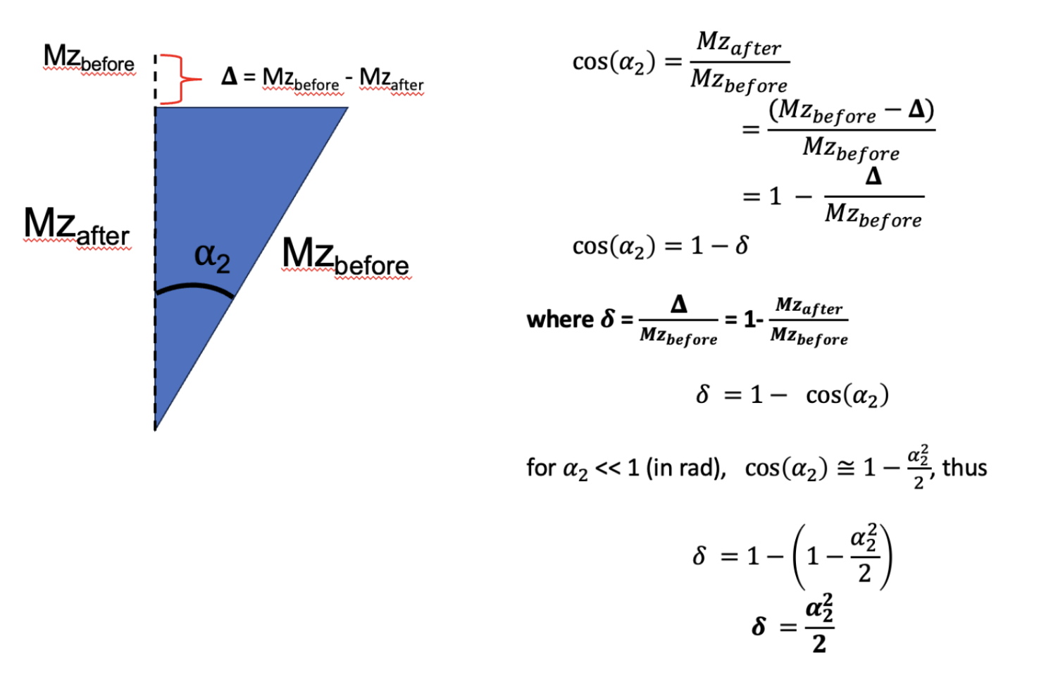
Figure 6.16:Demonstration through trigonometry of how following a small flip angle (eg MT saturation), the value represents the fraction of the reduction in longitudinal magnetization due to the pulse (bigDelta) relative to the value prior to the pulse (Mzbefore).
Before jumping into how to measure MTsat, let’s demonstrate some expected properties and values using known values from a simpler MTR experiment. From the MTR protocol in Brown et al., 2013 of the MTR section, =15 deg and TR = 0.03 s, so assuming a T1 at 1.5T (field strength that Brown used) of 0.55 s in healthy WM, so R1 = 1.8. First off, Figure 6.16 with no MT pulse (thus = 0) should converge close to the well-known SPGR equation (Eq. 6.8). Inputting the values in each equations, we get 0.0816A for [1], and 0.0815A, thus they are in close agreement. Next, we can get an estimated value of MTsat, using a known MTR value, the calculated S0 value (which we just did), and then solving [5] for using the MTR equation to bring everything together. Doing so is shown in Appendix A, from there and using our simulations in the MTR post with Brown et al., 2013 for healthier WM (MTR = 46%), we get an MTsat value of 4.92% ( = 0.0492), which is close to some reported MTsat values in the literature (Karakuzu et al. 2022). From there, and by definition of , the modeled in Figure 6.15 for this example is 18 degrees, confirming that earlier assumption that < 30 degrees for that approximation.
In that example, we used a known T1 value to extract MTsat using a two-measurement MTR experiment, but in practice this value is not known and varies per-pixel across tissues. Although we could use an additionally measured T1 map to do this, this can be time consuming depending on the method used. (Helms et al. 2008, 2010) thus demonstrated that with one additional T1w measurement that uses no MT preparation pulse but has different /TR than the MTon (MTw) and MToff (PDw) measurements used for MTR, that MTsat can be calculated analytically, and as a bonus a T1 map is also calculated in the process. (This makes sense, as the VFA T1 mapping sequence is often just two SPGR measurements with different values). Thus, using this three measurement protocol (MTw/PDw/T1w, which we’ll call the MTsat protocol), MTsat and T1 (1/R1) can be calculated analytically pixelwise using the following set of equations (derived from Eq. 6.5):
Remember, like MTR, MTsat is calculated from the equations above following the acquisition of the protocol images; no numerical fitting to a model is required. So effectively, the processing time to produce MTsat maps is the same as MTR, which is nearly instantaneous. Also, unlike MTR, which represents the steady-state signal difference due to the MT effect, MTsat represents the fraction of the longitudinal magnetization saturation caused by a single MT pulse within a TR, after a steady-state is achieved. Conventionally, it is represented as a percentage %, so MTsat is typically reported as . Note that MTR and MTsat are not expected to have the same values in magnitude despite both being represented as %, as they represent different changes. A major benefit of MTsat is that it’s expected to have less T1-dependency than MTR, as T1 (1/R1) is separately calculated and accounted for in the calculation of MTsat using the equations above. Although the MTsat metric is more robust against T1 changes, it is inherently sensitive to the MT preparation pulse properties (due to what MTsat physically represents, which is the saturation due to the MT pulse), and thus MTsat is not truly considered a fully quantitative metric as its value will change depending on the chosen protocol parameters and is not solely specific to the tissue properties or the field properties. Table 6.4 lists some MTsat protocol parameters that have been reported in the literature.
Table 6.4 :Some reported MTsat protocol parameters in the scientific literature (sources: Helms et al., 2008Weiskopf et al., 2013Campbell et al., 2018Karakuzu et al., 2022York et al., 2022)
| Helms 2008 | Weiskopf 2013 | Campbell 2018 | Karakuzu 2022 | York 2022 | |||
|---|---|---|---|---|---|---|---|
| Siemens | Siemens | Siemens | GE | Siemens | Siemens | ||
| T1w | FA | 15 | 20 | 15 | 20 | 20 | 18 |
| TR (ms) | 11 | 18.7 | 11 | 18 | 18 | 15 | |
| TE (ms) | 4.92 | 2.2–14.7 | - | 4 | 4 | 1.54/4.55/8.49 | |
| PDw | FA | 5 | 6 | 5 | 6 | 6 | 5 |
| TR (ms) | 25 | 23.7 | 30 | 32 | 32 | 30 | |
| TE (ms) | 4.92 | 2.2–14.7 | - | 4 | 4 | 1.54/4.55/8.49 | |
| MTw | FA | 5 | 6 | 5 | 6 | 6 | 5 |
| TR (ms) | 25 | 23.7 | 30 | 32 | 32 | 30 | |
| TE (ms) | 4.92 | 2.2–14.7 | - | 4 | 4 | 1.54/4.55/8.49 | |
| Offset (Hz) | 2200 | 2000 | 2200 | 1200 | 1200 | 1200 | |
| MT pulse shape | Gaussian | Gaussian | - | Fermi | Gaussian | Gaussian | |
| MT pulse length (ms) | 12.8 | 4 | - | 8 | 10 | 9.984 | |
| MT pulse angle (deg) | 540 | 220 | 540 | 540 | 540 | 500 | |
Simulations
In line with our previous MTR blog post, we employ the qMRLab qMT simulations to model MTsat measurements and subsequently calculate MTsat values from Eq. 6.7, Eq. 6.8, and Eq. 6.9. Table 6.5 lists the essential tissue parameters used for the simulations. Figure 6.17 plots the MTsat values that have been calculated for each protocol outlined in Table 6.4 , while also incorporating the relevant tissue parameters found in Table 6.5.
Table 6.5:Quantitative MT parameters in healthy and diseased human tissue reported for a study at 1.5 T Sled & Pike, 2001.
| Healthy cortical GM | Healthy WM | NAWM | Early WM MS lesion | Late WM MS lesion | |
|---|---|---|---|---|---|
| F | 0.072 ± 0.013 | 0.161 ± 0.025 | 0.15 ± 0.02 | 0.12 ± 0.02 | 0.094 ± 0.015 |
| kf | 2.4 ± 0.013 | 4.3 ± 1.0 | 4.9 ± 1.3 | 3.6 ± 0.8 | 2.7 ± 0.7 |
| R1,f (s-1) | 0.93 ± 0.2 | 1.8 ± 0.3 | 1.78 ± 0.4 | 1.52 ± 0.2 | 1.26 ± 0.3 |
| R1,r (s-1) | 1 | 1 | 1 | 1 | 1 |
| T2,f (ms) | 56 ± 8 | 37 ± 8 | 38 ± 7 | 43 ± 6 | 52 ± 9 |
| T2,r (μs) | 11.1 ± 8 | 12.3 ± 1.6 | 11.4 ± 1.4 | 10.3 ± 1.1 | 10.9 ± 1.4 |
Figure 6.17:MTsat values calculated from fundamental qMT tissue parameters for four different MTR imaging protocols.
It’s worth noting that MTsat values show a relatively wider range in values across protocols and tissue types (1% to 7%) when compared against our similar simulations for MTR (30%-60%). Additionally, note the change in order of magnitude of the values between MTsat (~5%) and MTR (~50%). As is demonstrated in the simulations above, MTsat values can be quite similar in both healthy and diseased tissues if different imaging protocols are used. So, for practical purposes, it’s recommended to use and compare MTsat values that were measured using a consistent imaging protocol (which, due to some proprietary pulse sequence designs, means that consistency will be best when using the same MRI vendor and version for the study). Nevertheless, some normalization techniques have been developed to make MTsat more useful in broader contexts.
To assess the relationship between MTsat and T1, we conducted simulations by varying T1 values as inputs for a specific protocol. In Figure 6.18, we present the resulting data, which includes calculated MTR (based on MT-on and PDw measurements), MTsat, and T1,meas values. As observed previously, MTR exhibits a high sensitivity to alterations in the tissue T1 values. Notably, the calculated T1 values closely mirror the input T1 values, evident in the identity line on the graph. MTsat shows minimal sensitivity to changes in T1, as even a ±30% variation in T1 values corresponds to only around a ±2% fluctuation in MTsat values.
Similarly, we can investigate the sensitivity of MTsat to B1, which varies substantially in the scanner at magnetic field strengths of 3T and above. In the human brain, B1 typically fluctuates the nominal flip angles within a range of -30% to 10% (Boudreau et al. 2017). Figure 6.19 displays the calculated MTR, MTsat, and T1 values using a range of B1 values +-30% to both the excitation and MT pulses. All three parameters demonstrate high sensitivity to changes in B1. Notably, while T1 is relatively insensitive to minor magnetic field variations, the calculated T1 values may deviate from accuracy. In contrast, the calculated MTsat inherently reflects the actual saturation induced by the MT pulse, which is directly proportional to B1. This relationship is expected since lower B1 values result in lower true MTsat values, which is particularly relevant when attempting to use MTsat as a biomarker for myelin content. To address this issue, an empirical equation Weiskopf et al., 2013 has been introduced to estimate the MTsat value that would have been measured if B1 values had been uniform across the brain, although it’s essential to emphasize that this is not a representation of the actual MTsat values the tissue experiences, but a means to standardize MTsat even in the presence of inhomogeneous B1 maps if/when RF transmit shimming isn’t done.
'mtsatb1.html'Figure 6.19:MTR/T1,meas/MTsat vs B1 values. Click button to compare values with or without B1-correction
5Appendix A
In reality, what is conserved and transferred during an MT experiment, is energy, and this energy is exhibited as non-zero magnetization under the correct conditions. Figure 6A-1 illustrates this. As is known from MR theory, the net magnetization of a population of spins at thermal equilibrium is a result of an excess (on the order of 10 ppm at 3T) of spins in the low energy level (spins aligned with the magnetic field) relative to the high energy level (spins anti-parallel to the magnetic field), with the energy level splitting (a) being due the nuclear Zeeman effect and for the free pool, has an difference E of (i.e. the energy corresponding to the resonance frequency, being the Planck constant). By applying an off-resonance frequency RF pulse (Δ), we can selectively transfer energy from the electromagnetic field to the restricted pool system such that some spins will jump from the low energy level to the high energy level (RF pumping, b), leaving the free pool undisturbed. This excess in energy that is now in the restricted pool spin population will then redistribute itself through several physical processes to reach a new system-wide equilibrium, such as energy transfer into heat through collisions, or spin exchange free pool spins through dipolar coupling or chemical exchange (Figure 6A-1a). This energy transferred to the free pool is represented by a slight reduction in the net magnetization of the free pool, which manifests as a decrease in the observed MR signal. This signal reduction occurs because the energy absorbed by the restricted pool (via the off-resonance RF pulse) results in fewer spins in the low-energy state in the free pool, thus reducing its longitudinal magnetization. Over time, the system will reach a new equilibrium state, where the magnetization of both the restricted and free pools reflects this redistributed energy.
In Figure 6A-1c (right), the new equilibrium state of the magnetization is shown, highlighting how the energy transfer process affects the magnetization of the free pool and, consequently, the overall MR signal. This phenomenon is central to magnetization transfer (MT) imaging, where the contrast in images is derived from the differences in energy transfer between different tissue types. The degree of MT contrast is influenced by factors such as the efficiency of energy transfer processes and the specific properties of the tissue, including the concentration and exchange rates of the restricted pool.
Ultimately, the conservation of energy and its transfer between different spin populations is what underlies the observable effects in MT imaging, allowing it to be used as a tool to probe tissue microstructure and composition.
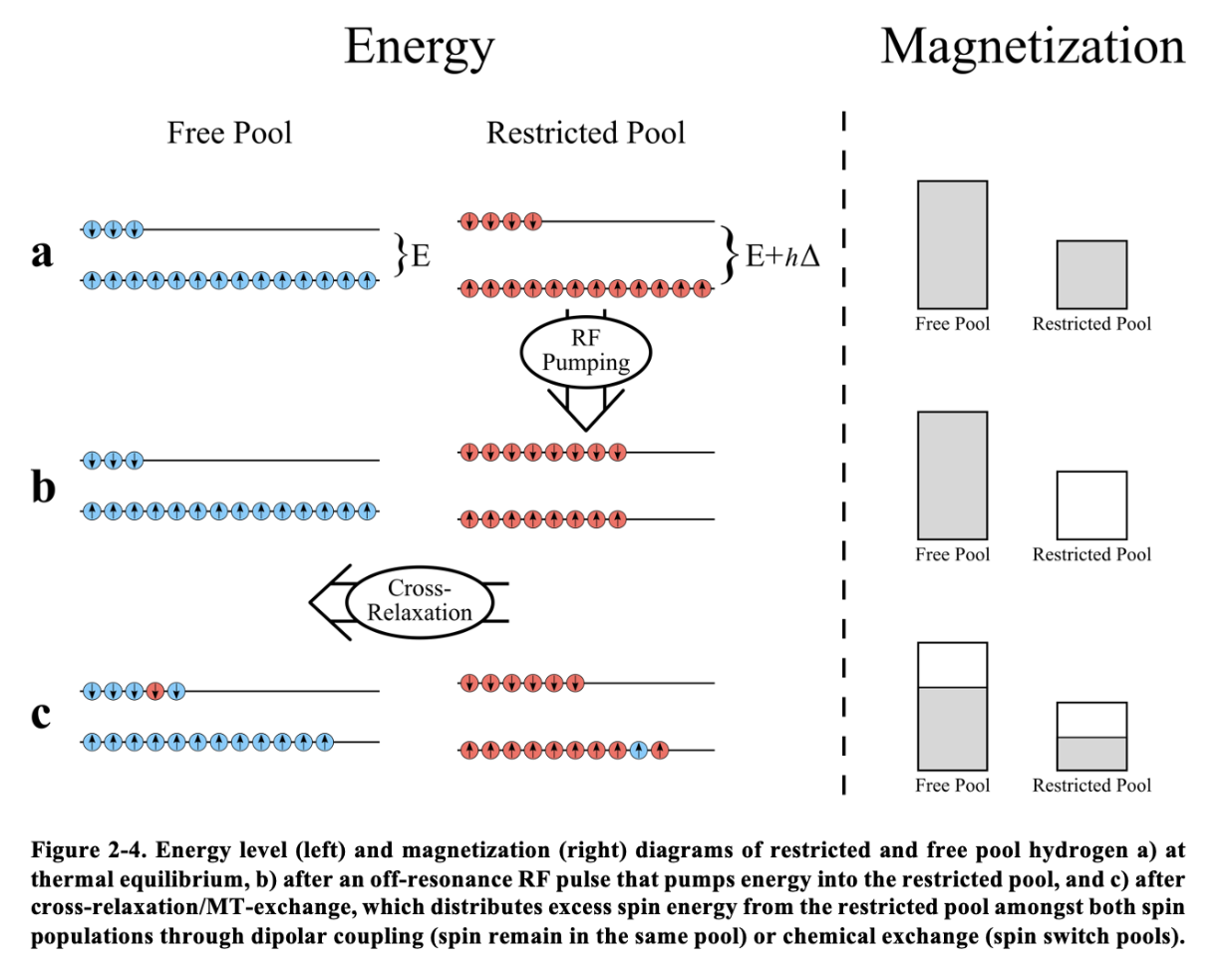
Figure 6A-1 :Thesis figure
6Appendix B
Derivation
From the MTR protocol in Brown et al., 2013 of the MTR section, =15 deg and TR = 0.03 s, so assuming a T1 at 1.5T (field strength that Brown used) of 0.55 s in healthy WM, so R1 = 1.8, we can calculate the signal from Eq. 6.6 of an experiment with no MT pulse ( = 0).
For an MT-weighted image, we get an equation as we don’t know ,
To simplify (and for reasons seen later), let’s define ,
We’d like to calculate the contribution from the MT pulse, δ. We can do this by using the measured MTR value for this protocol, which we simulated for in the previous blog post and found to be ~0.46. We can now use the MTR equation and substitute the S0 and SMT, and the solve for δ.
7Appendix C
So far we’ve explored a lot of the practical properties of MTsat, but have yet to explore what this parameter represents in reality. We begin this discussion by looking at how Helms et al., 2008 interpreted MTsat:
(figure or quote)
Thus, MTsat is interpreted as being the saturation (i.e. reduction in longitudinal magnetization) occurring from the pulse substituting the MT pulse (Figure 6.15 ) occurring within a single TR, after steady-state has been reached. A reminder: MTR, in contrast, is a steady-state image difference metric (not “within” a TR).
Simulating MTSat through qMRLab
To assess the validity of this MTsat interpretation, we employ Bloch simulations via qMRLab. These simulations should allow us to visualize the “MTSat value” both as it approaches and after reaching steady-state by quantifying the difference in longitudinal magnetization before and after the MT pulse. The main question we have is: can we find the MT saturation (δ) value directly using Bloch simulations, and how close does it approach the calculated MT saturation value from a three-measurement experiment (equations 7-9)?
Using some high-school geometry, we see how we can calculate MTsat (delta) from this difference, assuming (as Helms did) that the MT saturation causes a flip of a specific angle.
Figure 6A.1:Demonstration through trigonometry of how following a small flip angle alpha2 (eg MT saturation), the value represents the fraction of the reduction in longitudinal magnetization due to the pulse (bigDelta) relative to the value prior to the pulse (Mzbefore).
7.1Simulation 1: Revisiting MTsat Theory
In our first simulation, we use the qMRLab qMT-SPGR module to simulate steady-state signals from an MTsat experiment on healthy white matter tissues. We utilize tissue parameters from Sled & Pike, 2001 and an MTsat protocol derived from Karakuzu et al., 2022.
Code
clear all, close all, clc

%% Load protocol

fname = 'configs/mtsat-protocols.json';
fid = fopen(fname);
raw = fread(fid,inf);
str = char(raw');
fclose(fid);
val = loadjson(str);

protocols = val.karakuzu2022.siemens1

%% Load tissues

fname = 'configs/tissues.json';
fid = fopen(fname);
raw = fread(fid,inf);
str = char(raw');
fclose(fid);
val = loadjson(str);

tissue = val.sled2001.healthywhitematter;

%% T1 range

T1_true = 1

%% qMT-SPGR experiment

MTsats = zeros(1,length(T1_true))
MTRs = zeros(1,length(T1_true))
T1s = zeros(1,length(T1_true))


protocol = protocols.pdw

fa = protocol.fa
tr = protocol.tr/1000
te = protocol.te/1000
offset = protocol.offset
mt_shape = protocol.mtshape
mt_duration = protocol.mtduration/1000
mt_angle = protocol.mtangle

Model = qmt_spgr;
Model.Prot.MTdata.Mat = [mt_angle, offset];
Model.Prot.TimingTable.Mat(5) = tr ;
Model.Prot.TimingTable.Mat(1) = mt_duration;
Model.Prot.TimingTable.Mat(4) = Model.Prot.TimingTable.Mat(5) - (Model.Prot.TimingTable.Mat(1) + Model.Prot.TimingTable.Mat(2) + Model.Prot.TimingTable.Mat(3)) ;
Model.options.Readpulsealpha = fa;
Model.options.MT_Pulse_Shape = mt_shape

params = tissue{1}
x = struct;
x.F = params.F.mean;
x.kr = params.kf.mean / x.F;
x.R1f = 1/T1_true;
x.R1r = 1;
x.T2f = params.T2f.mean/1000;
x.T2r = params.T2r.mean/(10^6);

Opt.SNR = 1000;
Opt.Method = 'Bloch sim';
Opt.ResetMz = false;

[FitResult, Smodel] = Model.Sim_Single_Voxel_Curve(x,Opt); % NOTE: this uses a modified version of the qmt_spgr.m file where the additional output is included. Not all version of qMRLab has this; if yours doesn't, go to the file and add the additional function output accordingly.

%% Cleanup

%Smodel is the normalized MT-SPGR value, that is, the signal with the MT
%pulse on divided by the signal from the same sequence with the MT pulse
%off. Since in the MTsat experiment, the PD-weighted pulse sequence is the
%latter case above, we then define:

Signal_MT = Smodel;
Signal_PDw = 1;

%% Find scaling value for T1w signal


% Get PDw/T1w ratio from analytical

PDw_Model = vfa_t1;

params.EXC_FA = protocols.pdw.fa;
params.T1 = T1_true; % Could improve by caclulating T1meas from qMT values
params.TR = protocols.pdw.tr/1000; % ms

PDw_anal = vfa_t1.analytical_solution(params);

T1w_Model = vfa_t1;

paramsT1w.EXC_FA = protocols.t1w.fa;
paramsT1w.T1 = T1_true; % ms
paramsT1w.TR = protocols.t1w.tr/1000; % ms

T1w_anal = vfa_t1.analytical_solution(paramsT1w);

T1wPDw_ratio = T1w_anal/PDw_anal

%% Cleanup

% Since Signal_PDw = 1, then it's clear that

Signal_T1w = T1wPDw_ratio

%% Calculate MTsat from signals

Model = mt_sat;
FlipAngle =  protocols.pdw.fa;
TR =  protocols.pdw.tr/1000;
Model.Prot.MTw.Mat = [ FlipAngle TR ];
FlipAngle = protocols.t1w.fa;
TR =  protocols.t1w.tr/1000;
Model.Prot.T1w.Mat = [ FlipAngle TR];
FlipAngle =  protocols.pdw.fa;
TR =  protocols.pdw.tr/1000;
Model.Prot.PDw.Mat = [ FlipAngle TR];

data = struct();
data.MTw=Signal_MT;
data.T1w=Signal_T1w;
data.PDw=Signal_PDw;
FitResults = FitData(data,Model,0);
MTsats = FitResults.MTSAT
MTRs = FitResults.MTR
T1s = FitResults.T1
Output
MTsats =

    5.3428


MTRs =

   58.9758


T1s =

    1.0100
Our results closely align with expectations (T1 fitted ~= T1 input, MTR ~58, MTsat ~5%). Converting the MTsat value to ɑ2 (see [#mtsatFig3]), we find that the MTSat value corresponds to an equivalent excitation pulse of approximately 18.7 degrees. Through Helms’ interpretation, we infer that the MT pulse should be reducing the longitudinal magnetization by roughly 0.05 (ie Mz_after pulse - Mz_before pulse = 0.05).
7.2Simulation 2: Challenging MTSat Model Assumptions
Using the qMRLab Bloch simulations, we can calculate the difference in longitudinal magnetization before and after the MT pulse, and see if this corresponds to the MTsat value calculated above.
Let’s do that.
Code
Some modifications of the qMRLab code are needed to output the before/after magnetizations into a file.
clear all, close all, clc

%% Load Mz before and after for each TR

load('sim2.mat')

%% Plot Mz before and after for each TR

figure()
plot(Mz_before, 'r')
hold on
plot(Mz_after, 'b')
legend('Mz_{before}', 'Mz_{after}')

figure()
plot(Mz_before(end-10+1:end), 'r')
hold on
plot(Mz_after(end-10+1:end), 'b')
legend('Mz_{before}', 'Mz_{after}')

figure()
plot(1-Mz_after./Mz_before)
legend('1-Mz_{after}/Mz_{before}')

figure()
plot((1-Mz_after./Mz_before)*100)
legend('1-Mz_{after}/Mz_{before}')
From these simulations, we find that there is a 0.314% reduction in longitudinal magnetization before/after the MT pulse after a steady state is achieved, which is an order of magnitude smaller than the MTsat value we calculated earlier for this protocol and tissue parameters (~5%). Either the MTsat theory is wrong, or we’re missing something. Revisiting the pulse sequence ([#mtsatFig1]) and the MTsat model ([#mtsatFig2]), we notice that while the MTsat model assumes instant excitation for both pulses, in reality the MT pulse is relatively long (~10 ms, [#mtsatProtocolTable]). So, while there is a decoupling between MT saturation and relaxation in the MTsat model ([#mtsatFig2]), in reality (and in our simulations) there is relaxation occurring during the MT pulse, and we didn’t account for that in the above simulation.
7.3Simulation 3: T1 Correction During MT Pulse
In our third simulation, we account for the T1 relaxation during the MT pulse. To simplify the calculations, and like Helms did, we’ll assume a decoupling between the MTsaturation and relaxation and calculate the T1 relaxation recovery independently for the duration of the MT pulse. We’ll then remove this contribution from the Mzafter-Mzbefore we calculated earlier (0.314%).
Code
Some modifications of the qMRLab code are needed to output the before/after magnetizations into a file.
clear all, close all, clc

%% Load Mz before and after for each TR

load('sim2.mat')

%% Plot Mz before and after for each TR

figure()

figure()
plot((1-Mz_after./Mz_before)*100)
hold on
plot((1-(Mz_after-delta_Mz_T1relax)./Mz_before)*100)

legend('MTsat before T1 correction', 'MTsat after T1 correction')

figure()
plot((1-(Mz_after-delta_Mz_T1relax)./Mz_before)*100)
legend('1-Mz_{after}/Mz_{before}')
Upon excluding the T1 contribution, the disparity Δ in Mz values prior to and following the MT pulse increased to 2.1%, which is to say, that the MT contribution of this pulse leads to a reduction of Mz by 2.1%. This outcome aligns with the expected behavior, as T1 relaxation perpetually seeks to increase longitudinal magnetization towards its equilibrium value, which inversely impacts Δ. Consequently, the Δ we just calculated within a given TR is now closer to the initial MTsat calculation based on simulated measurements (2.1% compared to 5.34%). Nevertheless, it is apparent that some critical element eludes our simulations since we’ve only calculated only half of the anticipated value using our Bloch simulations.
7.4Considering Exchange and Relaxation after the MT Pulse
Once again, let’s compare the actual pulse sequence (Figure 6.14) and the Helms model (Figure 6.15 . In the MTsat model, all of the magnetization exchange contribution is concentrated into the second instantaneous excitation-saturation pulse . In the actual pulse sequence and in our Bloch simulations (Figure 6.14), there is exchange during the MT pulse (which we’ve calculated above), but also when the MT pulse is off (because the longitudinal free and restricted magnetizations are not at equilibrium - see Bloch-McConnell equations in our qMT blog post). So, it’s likely that the contribution of MT when the off-resonance pulse is off also needs to be accounted for, if we want to calculate the MTsat value directly within a TR in Bloch simulations. This additional MT exchange between the restricted and free pool likely causes a reduction in longitudinal free relaxation which is encapsulated in the MTsat value (which makes sense, from the diagrams of the two-pool model of MT).
7.5Simulation 3: MT contribution after the off-resonance pulse
To calculate this second contribution, we will calculate the difference in Mz between the end of the MT pulse and the end of TR (just prior to the next MT pulse), and just like we did earlier, we’ll also subtract the T1 component (assuming that MT and T1 are decoupled during this time). Note that MTsat is the reduction in magnetization relative to its value prior to the MT pulse, so we need to normalize this contribution by the initial Mz (the same one we used for the MT pulse contribution, at the start of TR). Appendix C extends the diagram from Figure 8 to include the MT contribution after the MT pulse, and although more complex, it demonstrates the need for the note in the previous sentence.
Code
Some modifications of the qMRLab code are needed to output the before/after magnetizations into a file.
clear all, close all, clc

%% Load Mz before and after for each TR

load('sim2.mat')

%% Plot Mz before and after for each TR

figure()

figure()
plot((1-(Mz_after-delta_Mz_T1relax)./Mz_before)*100)

hold on
plot((1-(M0_remainingTR_free-delta_Mz_T1relax_remaining)./Mz_before)*100)
plot((1-(Mz_after-delta_Mz_T1relax)./Mz_before)*100+(1-(M0_remainingTR_free-delta_Mz_T1relax_remaining)./Mz_before)*100)

legend('MTsat contribution from MT pulse event', 'MTsat contribution from cross-relaxation event', 'Total MTsat for TR')
These simulations show through Bloch simulations that the sum of the MT contribution during and after the off-resonance pulse (with the T1 relaxation component removed) leads to a reduction in longitudinal magnetization of 5.49%, very close to the 5.34% that was calculated using the Helms model of MTsat in Eq. 6.7, Eq. 6.8, and Eq. 6.9. A slight overestimate still remains, but this difference is likely impossible to consolidate, as there will always be a difference between the actual MT exchange (where both MT and T1 are counteracting each other at all times) and the modeled MTsat exchange (where instantaneous pulses are assumed, so the MT and T1 contribution are completely separated in this theory).These simulations should however show that the MTsat contribution is not restricted to only the difference in Mz resulting after the effects of the MT pulse, but also to the cross-relaxation occurring between pools in the absence of the MT pulse.
7.6Interpreting MTSat
In conclusion, our reevaluation of MTSat suggests that it does not model solely the fractional saturation due to the MT pulse within a single TR, as conventionally understood. Instead, MTsat appears to represent the fractional saturation arising from the entire MT contribution during a TR, that is to say, both the MT pulse and the subsequent MT exchange between the two pools that takes place after following the off-resonance pulse. This subtle reinterpretation may challenge existing interpretations, as a greater contribution results from the exchange after the MT preparation pulse due to cross-relaxation caused by the perturbing MT pulse. This analysis highlights the power of open-source qMRI tools like qMRLab in fostering deeper understanding within the field.
Through a meticulous examination of MTSat, we encourage the scientific community to engage in further discussions and research, potentially leading to more refined models and insights into this crucial aspect of MRI physics in modelling tissue components that are difficult to measure directly, such as the semi-solid myelin sheets.
8Exercises
- Wolff, S. D., & Balaban, R. S. (1989). Magnetization transfer contrast (MTC) and tissue water proton relaxation in vivo. Magn. Reson. Med., 10(1), 135–144.
- Henkelman, R. M., Huang, X., Xiang, Q. S., Stanisz, G. J., Swanson, S. D., & Bronskill, M. J. (1993). Quantitative interpretation of magnetization transfer. Magn. Reson. Med., 29(6), 759–766.
- Santyr, G. E. (1993). Magnetization transfer effects in multislice MR imaging. Magnetic Resonance Imaging, 11(4), 521–532. https://doi.org/10.1016/0730-725X(93)90471-O
- Assländer, J., & Flassbeck, S. (2025). Magnetization transfer explains most of the T1 variability in the MRI literature. Magnetic Resonance in Medicine, 94(1), 293–301. https://doi.org/10.1002/mrm.30451
- Assländer, J. (2025). Sensitivity of literature T1 mapping methods to the underlying magnetization transfer parameters. https://arxiv.org/abs/2509.13644
- Sled, J. G. (2018). Modelling and interpretation of magnetization transfer imaging in the brain. Neuroimage, 182, 128–135.
- Schmierer, K., Scaravilli, F., Altmann, D. R., Barker, G. J., & Miller, D. H. (2004). Magnetization transfer ratio and myelin in postmortem multiple sclerosis brain. Ann. Neurol., 56(3), 407–415.
- Schmierer, K., Tozer, D. J., Scaravilli, F., Altmann, D. R., Barker, G. J., Tofts, P. S., & Miller, D. H. (2007). Quantitative magnetization transfer imaging in postmortem multiple sclerosis brain. J. Magn. Reson. Imaging, 26(1), 41–51.
- Fornari, E., Maeder, P., Meuli, R., Ghika, J., & Knyazeva, M. G. (2012). Demyelination of superficial white matter in early Alzheimer’s disease: a magnetization transfer imaging study. Neurobiol. Aging, 33(2), 428.e7-19.
- Chen, Z., Zhang, H., Jia, Z., Zhong, J., Huang, X., Du, M., Chen, L., Kuang, W., Sweeney, J. A., & Gong, Q. (2015). Magnetization transfer imaging of suicidal patients with major depressive disorder. Sci. Rep., 5(1), 9670.
- Sled, J. G., & Pike, G. B. (2001). Quantitative imaging of magnetization transfer exchange and relaxation properties in vivo using MRI. Magn. Reson. Med., 46(5), 923–931.
- Helms, G., Dathe, H., Kallenberg, K., & Dechent, P. (2008). High-resolution maps of magnetization transfer with inherent correction for RF inhomogeneity and T1 relaxation obtained from 3D FLASH MRI. Magn. Reson. Med., 60(6), 1396–1407.
- Zheng, Y., Lee, J.-C., Rudick, R., & Fisher, E. (2018). Long-term magnetization transfer ratio evolution in multiple sclerosis white matter lesions. J. Neuroimaging, 28(2), 191–198.
- Seiberlich, N., Gulani, V., Campbell-Washburn, A., Sourbron, S., Doneva, M. I., Calamante, F., & Hu, H. H. (Eds.). (2020). Quantitative magnetic resonance imaging. Academic Press.
- Cabana, J.-F., Gu, Y., Boudreau, M., Levesque, I. R., Atchia, Y., Sled, J. G., Narayanan, S., Arnold, D. L., Pike, G. B., Cohen-Adad, J., Duval, T., Vuong, M.-T., & Stikov, N. (2015). Quantitative magnetization transfer imagingmadeeasy with qMTLab: Software for data simulation, analysis, and visualization. Concepts Magn. Reson. Part A Bridg. Educ. Res., 44A(5), 263–277.