1Introduction
The main magnetic field (B0) plays a crucial role in MRI, dictating the precessional frequency of spins and establishing the bulk magnetization that determines image signal-to-noise ratio. However, imaging reconstruction techniques assume a perfectly homogeneous B0 field, an assumption that rarely holds true in practice. B0 inhomogeneities can lead to significant image artifacts including signal loss, geometric distortions Jezzard & Balaban, 1995, poor fat saturation Anzai et al., 1992, and spectral linewidth broadening in MR spectroscopy. These field variations arise from multiple sources including hardware imperfections during manufacturing Webb, 2016 and magnetic susceptibility differences at tissue interfaces Schenck, 1996.
Accurate mapping of B0 field variations is essential for both prospective correction through active shimming and retrospective correction of acquired data. B0 maps enable compensation for geometric distortions in techniques like EPI Jenkinson et al., 2012, recovery of signal decay for T2* mapping An & Lin, 2002, and form the foundation for quantitative susceptibility mapping (QSM) to characterize tissue magnetic properties.
This chapter explores the fundamental principles and advanced methodologies of B0 field mapping. We begin with the dual-echo phase difference technique, the most widely adopted approach that leverages the linear accumulation of phase over time to compute field maps through simple phase subtraction. While conceptually straightforward, this method faces challenges with phase wrapping artifacts and sensitivity to noise Brown et al., 2014, which we address through comprehensive discussion of both temporal and spatial phase unwrapping techniques. Building on these foundations, we examine multi-echo field mapping approaches that provide enhanced accuracy through improved phase unwrapping capabilities, as well as specialized methods for real-time field mapping and mitigation of eddy current effects. Throughout, we emphasize practical considerations for protocol optimization and the relative strengths of each technique for different clinical and research applications.
2B0 inhomogeneities
The main magnetic field, also called the B0 field, plays a crucial role in MRI. It dictates the precessional frequency of the spins and sets-up the bulk magnetization, which plays an important role in the image signal-to-noise ratio. Moreover, the radio frequency coils, tuned to the B0 field, are responsible for flipping the spins in the transverse plane and for acquiring the signal. However, imaging reconstruction techniques assume a perfectly homogeneous B0 field to reconstruct the signal from k-space data. An inhomogeneous B0 field can lead to image artifacts such as signal loss, distortions Jezzard & Balaban, 1995, poor fat saturation Anzai et al., 1992 and many other image artifacts. In extreme cases, it can completely hinder the ability to create an image. B0 inhomogeneities are also problematic for MR spectroscopy (MRS), because they widen the spectral linewidth.
When a subject is introduced in the scanner, the static B0 field can be rendered more homogeneous through a technique called active shimming. Active shimming sends the appropriate amount of current through specific gradient and shim coils, in order to generate a magnetic field that will compensate for the existing (inhomogeneous) magnetic field. This procedure requires precise and accurate mapping of the B0 field. B0 maps show the difference between the current field and the expected field, and are typically displayed in units of magnetic field strength (Tesla [T]), precessional frequency (Hertz [Hz]) or in parts per million (ppm). Eq. 5.1 can be used to convert from the different units.
where , and represent the actual precessional frequency, the Larmor frequency and the difference between current and the Larmor frequency () respectively. B, B{sub}0 and Δ B all have similar interpretations as , and but are in units of field strength (T). The relationship between frequency and field strength can be found using the well known Larmor equation (). is the field offset in ppm.
Figure 5.1 shows typical brain magnitude, phase, and B0 field map images of a brain in a 3 T scanner.
Figure 5.1:Magnitude image of the reconstructed MRI signal acquired at 3 T (A), the phase in radians (B), and a computed field map in Hz (C), 𝜇T (D) and ppm (E). The dropdown can be used to select between the different images.
Sources
2.1Hardware
Although scanner manufacturers try to make magnets that are as homogeneous as possible, they are far from perfect. The manufacturing process requires many kilometers of superconducting wire to be wound to create the main magnet and can lead to inhomogeneities due to manufacturing tolerances. Moreover, large metal objects near the scanner can interact with the field created by the scanner and impact the resulting field within the scanner. This is a more important problem with higher field strength. During the installation process, the empty bore is homogenized in a process called passive shimming. During this process, small ferromagnetic pieces are introduced in the scanner at optimized locations to produce a field that counteracts the inhomogeneities. Hardware inhomogeneities are relatively small (less than 1 ppm Webb, 2016).
Specialized equipment such as field probes Dietrich et al., 2016 (e.g.: Skope Magnetic Resonance Technologies, LLC) can be used to evaluate the B0 field of the scanner while it is being installed. This equipment can also be used after installation because it is more precise than B0 field maps and offers better field temporal resolution, allowing the ability to observe eddy currents created from gradient switching.
During an imaging session, heating of the different components and of the main magnet can lead to temperature-dependent changes in the B0 field. These can be observed by a frequency drift in the field. As an example, a ~0.4Hz/min has been observed in MRS at 3T but depends on multiple factors Academic Press, 2021. Modern scanners usually have systems in place to evaluate and correct for this drift El-Sharkawy et al., 2006.
2.2Magnetic susceptibility
Materials have a property called magnetic susceptibility () that reflects their ability to become magnetized in response to an external magnetic field Schenck, 1996. The change in magnetic field Bz (the subscript “z” is shown to make it explicit that we are referring to the component parallel to the B0 field) is proportional to the magnetic susceptibility value, the magnetic field strength, and can be affected by the geometry and location of the tissues. It can be modeled as a convolution of the difference in magnetic susceptibility with the component parallel to the magnetic field induced by a unit magnetic dipole () in spherical coordinates where is the position vector and is the angle with B0 Rochefort et al., 2008.
The dipole kernel (d) is illustrated in Figure 5.2 along with the dipole kernel (D) in the k-space domain often used in QSM.
Figure 5.2:Dipole kernel (d) in the image domain as well as in the k-space domain (D).
When a subject is introduced in the scanner, it interacts with the B0 field and distorts it. Therefore, a perfectly homogeneous field in an empty bore will usually have an inhomogeneous B0 field once a patient is introduced. This is the reason why active shimming is required when a patient is introduced in the scanner. Although these inhomogeneities happen everywhere in the body, stronger field variations occur at the boundaries of strong susceptibility differences such as air (slightly paramagnetic: ) and water/tissue (diamagnetic: ).
The following figure shows different susceptibility distributions in ppm for a homogeneous cylinder within a larger homogeneous cylinder placed in a homogeneous background (top) and a brain (bottom). The corresponding B0 field maps are simulated at 7 T and shown in Figure 5.3. In the brain, the B0 field inhomogeneities are dominated by air-tissue boundaries. On the right-hand panel, the slow varying spatial variations (also called background field) were removed to show the local field variations.
Figure 5.3:Cylinder (top) and brain (bottom) of susceptibility distributions (left), simulated B0 field map (middle) and the B0 field map with the background field removed (right). An in-vivo susceptibility map was used for the brain and was surrounded with air. Note that this simplistic representation still shows the field map being dominated by air-tissue interfaces even though the spatial characteristics of the field are not perfectly representative of reality. An in-vivo field map can be seen in Figure 5.9.
Effects on signal
To excite the spins in the transverse plane, a carrier frequency tuned to the Larmor frequency is used by the transmit coil. If the frequency of the spins does not match the excitation frequency, it results in a suboptimal tip of the spins in the transverse plane. If the frequency of the spins varies across the ROI, the flip angle is affected differently across the image Wang et al., 2006.
When a signal is acquired, it is demodulated to remove the carrier frequency (Larmor frequency) from the signal. An example of a FID is shown in Figure 5.4. The number of species represent the number of isochromats in the simulation. An isochromat represents an ensemble of spins with the same properties rotating at the same Larmor frequency. For a single isochromat, if the acquired signal and demodulation frequency perfectly match, the T2 signal can be recovered. If the carrier frequency is different from the expected frequency (such as when there are inhomogeneities), the demodulation introduces low-frequency variations. A non-homogeneous sample is also shown featuring many isochromats. Alternatively, a homogeneous sample with a non-homogeneous B0 field could be simulated as well and would have a similar shape as the one with multiple species. In that case, the difference from the T2 curve would reflect T2* () effects. During the relaxation process, spins precessing at different frequencies, due to the presence of B0 inhomogeneities, will give rise to phase offsets between the spins within a voxel. This intravoxel phase dispersion leads to signal decay.
Figure 5.4:FID curves with signal demodulation at Larmor frequency (single species), at two different frequencies (Larmor and offset frequency, two species) and at multiple frequencies (Larmor frequency and many other offset frequencies, multiple species). The resulting shape of the graphs depends on the relative amplitudes and frequencies.
B0 inhomogeneities can lead to distorted k-space trajectories during the readout gradient. This effect is worse during further k-space traversal due to the compounding of the errors. When inhomogeneities are present, the frequencies of the spins are altered. The one-to-one relationship between frequency and spatial location (required to obtain accurate spatial correspondence) is broken. This leads to geometric distortions. Figure 5.5 shows an animation of the filing of k-space of an EPI sequence using bi-polar readouts. A theoretical trajectory is shown as well as a trajectory where a constant parasite gradient in the phase encoding direction has been added. One can observe the trajectory differences.
Figure 5.5:K-space trajectory of an EPI sequence using bi-polar readout gradients (blue). A constant gradient in the positive phase encoding direction is applied to simulate inhomogeneities (red). The trajectory with the parasite gradient deviates from the theoretical trajectory. All encoding gradients (G) are instantaneously applied at 40 mT/m. A parasit Gp,phase of 0.1mT/m (G/Gp,phase=0.25%) is added to simulate inhomogeneities. 64 encoding steps are used in both the frequency and phase encoding directions but only one in five phase encoding lines is shown for visualization purposes.
Radiofrequency (RF) pulses can also be affected by an inhomogeneous B0 field. During slice selection for example, the RF pulse excites a range of frequencies that can be mapped to spatial locations by applying a linearly evolving magnetic field along the slice direction. For a perfectly transverse acquisition, the resulting B0 field can be expressed by (). If B0 inhomogeneities are present (), the excited slice profile can be distorted or offset from the expected location. When B0 inhomogeneities are very inhomogeneous, they can also disrupt frequency-selective RF pulses such as fat saturation pulses. There are also other effects such as ringing artifacts, blurring, and ghosting that can occur.
All of these effects can be minimized with B0 shimming. To do so, a map of the B0 field can be acquired. In addition to shimming, B0 mapping is important for other techniques that will be discussed later. The next section will show how to perform B0 mapping using two echoes.
3Dual echo B0 mapping
B0 mapping estimates the B0 field from the expected field for every voxel. These B0 maps can be used to perform prospective B0 shimming to minimize B0 inhomogeneities Jezzard & Balaban, 1995, they can be used to retrospectively correct for geometric distortions (FSL FUGUE Jenkinson et al., 2012Smith et al., 2004) (e.g.: for EPI), or to perform retrospective correction for k-space readout trajectory (e.g.: for spiral readout). Moreover, they can be used for retrospective recovery of enhanced signal decay An & Lin, 2002Alonso-Ortiz et al., 2017, for T2* mapping and they are also vital to quantitative susceptibility mapping (QSM) where the goal is to map the susceptibility of the subject.
One of the most simple and widely adopted techniques used to perform B0 mapping is the 2-echo phase difference technique. This technique is faster and simpler than most other alternatives. Before we dive into the technique, let’s dip our toes in some theory.
Signal Theory
In the ideal case, spins rotate at the Larmor frequency, shown in blue in Figure 5.6. In the presence of field inhomogeneities, the frequency of the spins (shown in red) is different and is proportional to the field inhomogeneities. Both the laboratory and rotating frame of reference are shown. Importantly, note that the Larmor frequency phase appears stationary in the rotating frame of reference.
Figure 5.6:Two spins rotating (one at the Larmor frequency (), one at a lower frequency). A view of the spins in the transverse plane (left) and of their phase (right) is shown. A dropdown is available to select between the laboratory frame and the rotating frame of reference.
The phase () evolution follows the following equation (not considering transient effects such as eddy currents) in the rotating frame of reference.
where x,y,z are the coordinate locations, t is time, is the gyromagnetic ratio, B0 is the B0 field offset (Tesla) and is an initial constant phase offset (e.g.: coil induced, material induced through local conductivity/permittivity). We can observe phase evolution through time in Figure 5.7 by looking at phase data acquired in the brain at progressively longer echo times. The phase at a single voxel changes linearly (not considering transient effects). Note that the sharp variations forming vertical lines in the previous figure are called phase wraps and occur because the phase is defined over - to . Phase-wrapping effects will be discussed in more detail in the following section. Wraps can also occur spatially as sharp variations as seen in the following figure. Note that the longer the echo times, the more wraps there are.
Figure 5.7:Phase shown at different echo times. The slider can be used to show the phase that would be acquired at different echo times.
MRI manufacturers do not all output phase data by default. It should be possible to toggle the output of phase data on all MRI systems. It can also be computed from real/imaginary data using Eq. 5.4.
where is the phase operator.
As phase changes linearly with time (t) and with the field offset (B0), it is possible to acquire two phase images at two different echo times and compute B0(x,y,z).
where TE1 and TE2 are the echo times, and TE = TE2- TE1. To compute the phase offset , phase subtraction is necessary. The complex difference can be used to keep the phase between to , although other phase difference techniques are also possible.
In some sequences, the phase images are exported as a single phase difference image .
Single Frequency Population
To build intuition about field maps, let us imagine a sample at a constant offset frequency from . Note that this simplistic representation of the field typically does not occur due to how the susceptibilities of the neighboring regions interact with one another to create the B0 field offset (see the B0 inhomogeneity section, but is shown as such for learning purposes. The sample is shown as a circle in Figure 5.8. As the frequency is not at the Larmor frequency, phase accumulation is observed at the different echo times and a phase difference map can be computed. The B0 field map is then calculated using the echo times. Note that if TE is too long, the phase could make more than a half revolution between the two echo times resulting in an erroneous B0 field estimation. This is because phase is defined over to and the sampled points should respect the Nyquist criteria. In practice, this example field (constant offset) could easily be corrected by adjusting the transmit and receive frequency of the scanner.
Figure 5.8:Different images of a homogeneous cylinder field offset showing a simulated phase at two echo times, the calculated phase difference image and the computed B0 field map.
Multi Frequency Population
A brain dataset is used to show a concrete example of a field map that could be acquired in practice. Figure 5.9 shows two phase images where phase accumulation is shown due to frequency offsets that vary spatially. As mentioned previously, phase wraps are visible where phase transitions from to and will be discussed in more detail in the next chapter. The phase difference and B0 field maps are also shown. Note that taking the phase difference eliminates the wraps in this example, however, there could be residual wraps when the field is more inhomogeneous.
Figure 5.9:Two phase images, a phase difference and a B0 field map. Phase wraps are visible where the phase transitions from to .
Benefits and Pitfalls
When acquiring a field mapping sequence, many parameters will affect the resulting images. A minimum of two phase images is required to compute B0 field maps, as the initial phase is generally not known and non-zero. Multi-echo field mapping with more than two echoes will be discussed in the the advanced B0 mapping section.
These phase maps can be acquired by many sequences. The general principle includes the use of sequences that cause accumulation of phase. This can be done using GRE sequences or using spin-echo sequences with asymmetric echoes (e.g.: first echo at the spin echo and second echo shifted by 1-2 ms to create an accumulation of phase caused by B0 inhomogeneities). The sequence parameters are chosen such that the data does not suffer much from distortions and other artifacts caused by B0 inhomogeneities. High bandwidth, thin slices and multi-shot sequences are therefore preferred Akcakaya et al., 2022. This means EPI sequences are generally not used for field mapping because of their sensitivity to B0 inhomogeneities.
When acquiring multiple echoes, the readout direction of the even echoes can be chosen to either be in the same direction (monopolar) as the odd echoes or in opposite directions (bipolar). Using opposite directions can slightly reduce TE, but doing so can cause a slight misregistration between the even and odd echoes and we therefore recommend using readouts in the same direction.
The standard deviation of the phase () is inversely proportional to the SNR of the magnitude image (SNRmag) Brown et al., 2014.
A high SNR image will therefore provide a more reliable phase image. With this in mind, the main parameters to choose are the echo times. The first echo time is usually chosen to be quite fast to maximize SNR and minimize phase wraps. The choice of the second echo time is then chosen according to many factors. i) Fat has ~3.35 ppm frequency offset from water. This can cause errors in the fieldmap measurement, where a chemical shift is mistaken for a field shift near and within fatty tissues. TE can be chosen so that fat and water are in phase and reduce this problem (~2.34ms at 3T). Note that different fat components have different chemical shifts. These values are given as first estimates. ii) Longer TE maximizes the difference between the phase measurements and can provide a better estimate if SNR is still sufficient. iii) Shorter TE minimizes the number of wraps and therefore reduces errors due to unwrapping. If the field offset is known, a maximum TE can be calculated to yield no phase wrapping.
As echoes are usually acquired in rapid successions to avoid phase wrapping, rapid gradient switching is required which leads to eddy currents that can impact the acquired phase data. To mitigate the issue, a single echo per RF pulse can be acquired. A dual-echo sequence would have twice the number of RF pulses (alternating between acquiring both echoes) but allows slower gradient switching and removes eddy currents effects from the gradient work of the first echo on the second echo. However, this technique requires longer scan time.
As seen in this section, phase wrapping can be an issue, as phase is defined over . The next section deals with this problem.
4Phase Unwrapping
Phase unwrapping stems from the fact that phase can only be measured over the range of to . If the measured phase crosses from to , a “wrap” is observed as a jump where in reality, the phase was smoothly varying. In the context of MRI, phase wrapping occurs when measuring phase data that varies by more than within the region of interest. In reality, the number of rotations that a spin can have done is not limited to a single revolution. To accurately recover the true phase information, unwrapping is necessary.
There are two main families of unwrapping techniques. Temporal unwrapping techniques use temporal information from different phase time points and the assumption that the difference between time points is smoothly varying (offset less than ) to correct for phase jumps that can occur in time. Spatial unwrapping uses spatial information and relies on the fact that neighboring voxels should be smoothly varying to identify and correct for jumps.
Temporal Unwrapping
Temporal unwrapping uses multiple time points (>=2) to unwrap the image. By acquiring phase data that vary by at most to , the difference between 2 echoes (using complex difference) yields an unwrapped image free of wraps. Eq. 1 describes the field offset () experienced during TE in the presence of field inhomogeneities.
If we assume a maximum field offset of 1 ppm at 3T (~127 MHz), we can calculate a maximum field offset () of 1 µT or 127 Hz. The Nyquist criteria can be used to calculate the maximum echo time difference (TE) required to satisfy the no-wrapping requirement in the phase difference image (). Table 5.1 shows TE for multiple field strength assuming inhomogeneities of 1 ppm. As shown, the echo spacing is B0 dependent, as higher field offsets are observed at higher field strengths.
Table 5.1:Maximum echo time required to respect the Nyquist criteria for different field strengths for ΔB0 of 1 ppm.
B0 (T) | deltaTE (ms) |
|---|---|
0.064 | 183.39 |
0.1 | 117.37 |
0.3 | 39.12 |
1.5 | 7.82 |
3 | 3.91 |
7 | 1.68 |
If a longer TE is selected, or if the inhomogeneities are bigger than originally anticipated in some parts of the image, the phase difference image could also have wraps, and spatial unwrapping would be necessary.
Temporal unwrapping can also be performed without phase difference. Figure 5.10 shows the phase of a voxel acquired at four echo times in blue. Note that the last echo time is wrapped (i.e.: the phase rotated by more than and “wrapped” to the positive side). With the assumption that phase does not vary by more than , we can unwrap the phase by, in this case, subtracting from the acquired phase to recover the true phase (in red). A linear fit is shown in green. Note that the slope would represent the field map value.
Figure 5.10:Four phase voxels acquired at different echo times (blue). The phase is unwrapped temporally and plotted, which in this case changes the phase of the 4th echo (red). A linear fit is also shown (green).
Spatial Unwrapping
Spatial unwrapping uses the spatial characteristics of images to unwrap the data. The wrapped image should vary smoothly. Spatial unwrapping typically uses a region-growing algorithm which identifies and rectifies where there are offsets greater than . An example of a 1D signal of a linearly evolving phase is shown in Figure 5.11 to illustrate the phase that we would want to recover from the wrapped phase that would be acquired through space.
Figure 5.11:1D example of a wrapped phase (blue) with the true phase (red)
A more complex example is shown in Figure 5.12 where phase varies spatially in a non-linear fashion. When the signal is unwrapped, different solutions are expected. These solutions vary by . Its cause and potential remedy are described in the following section.
Figure 5.12:A more complex example of a signal wrapped and unwrapped. Note that three possibilities are possible when unwrapping, depending on which part of the signal is selected to be the true phase. The slider can be moved left to right to show the wrapped and unwrapped data.
A common issue with spatial unwrapping which stems from region growing algorithms is that the region of interest needs to be defined in a single region, or there can be a offset between regions. Moreover, region growing algorithms usually require thresholding so that noise is not unwrapped.
A 2D example of wrapped and unwrapped simulated data is shown in Figure 5.13. The concept can be expanded to 3D data as well. Note that more wraps result in higher field inhomogeneity.
Phase unwrapping ambiguity
There is ambiguity to unwrapping and a choice needs to be made regarding the true signal (see Figure 5.12). If the wrong one is selected, this creates a offset from the true phase. When unwrapping a single phase volume, an educated guess can be made by calculating the average phase in the ROI and expect that to be close to 0 (we assume here that a good frequency shim was first performed in the ROI). n is chosen and the offset is removed from the unwrapped phase map such that the average phase in the ROI is close to 0. Note that this is not a perfectly robust solution because phase is also affected by other factors such as the receive coil, RF pulse and eddy currents which could cause the average phase offset to deviate from 0. Fortunately, phase difference images are more reliably unwrapped since some of the phase offsets are constant in both phase images and are removed when performing the phase difference resulting in a phase offset closer to 0.
If multiple echoes are acquired, a combination of spatial and temporal unwrapping may be necessary. Multi-echo field mapping is discussed in the following section. Note that with appropriate selections of the echo times, the offset ambiguity can be remedied.
Problematic phase map properties
Phase maps sometimes have wraps that are not possible to unwrap with traditional phase unwrapping techniques. One example is shown in Figure 5.14. Phase singularities, also called poles or open ended fringe lines, hinder the abilities of unwrappers to get an accurate unwrapped phase. As can be seen in the following figure, there are two points where the phase is ambiguous. When unwrapping spatially, if two points are selected arbitrarily in the ROI, one would expect that all possible paths linking both points to cross the same number of wraps. Otherwise, crossing a different number of wraps results in ambiguous phase values. Counting wraps can be done by counting the sharp phase transitions where to (black to white) results in +1 wrap and to (white to black) results -1 wrap. However, phase singularities create paths that have a different number of wrap crossings, resulting in ambiguous phase values. Figure 5.14 is used as an example to illustrate the above statements. When unwrapping from point A to B, the left path crosses no wraps and would therefore expect the phase to go from to , however, the right path crosses a wrap and would therefore expect to go from to . This is problematic as the phase becomes ambiguous. Phase singularities are usually a result of a poor coil combination process. There are some techniques to mitigate the issue, but the main solution is to correctly combine the coil maps to avoid the singularities altogether.
Figure 5.14:Synthetic phase data showing two phase singularities. The red paths show two different paths a region growing algorithm could use to go from point A to point B. The left path does not cross a phase wrap whereas the right path crosses a phase wrap. This yields an ambiguous phase result.
Software
Laplacian unwrapping can be very robust even with highly wrapped images but does so at the expense of accuracy. It typically unwraps with an error of low spatial variability. This can be a perfectly reasonable unwrapping technique for some applications such as QSM where the background field (low spatial variability) is subsequently removed. However, in applications such as shimming or qMRI where the accuracy is important, Laplacian unwrapping is not recommended.
Other unwrapping algorithms and softwares are listed below.
PRELUDE: Spatial unwrapping technique using region growing algorithm Jenkinson, 2003. SEGUE: Spatial unwrapping technique based on similar principles to Prelude with optimizations to improve the speed Karsa & Shmueli, 2019. BEST PATH: 3D unwrapping algorithm using spatial information to assess the quality of the phase data and unwrap high quality regions first. Abdul-Rahman et al., 2007 ROMEO: Unwrapping technique using temporal and spatial information to guide the path of unwrapping Dymerska et al., 2021. UMPIRE:Temporal unwrapping technique using unevenly spaced echoes to accurately unwrap phase images. This technique requires three or more echoes Robinson et al., 2014.
5Advanced B0 Mapping Methods
Although dual-echo field mapping can be used for many applications, more advanced B0 mapping techniques are available depending on the use-case. Multi-echo field mapping, which makes use of more echoes, can be used to increase the accuracy of the computed field map. This can be useful for qMRI, shimming, or QSM, where the goal is to gather field information to map the susceptibility of the tissues. QSM is sensitive to small local variations, therefore a more accurate approach can be beneficial. This section also discusses fast B0 field mapping in the context of capturing B0 variations due to air differences generated by breathing. B0 maps can be affected by eddy currents and a section is dedicated to their reduction.
Multi-echo B0 mapping
Multi-echo field mapping (three or more echoes) makes use of more echo times than the dual-echo standard field map. With more time points, the field maps can be expected to be more accurate. All benefits and pitfalls of dual echo B0 mapping apply in multi-echo field mapping, with the added criteria that the later echoes should have enough signal to provide a benefit to the technique. As seen in the dual echo B0 mapping section, the phase generally evolves linearly with respect to time. Another way to look at B0 field mapping is realizing that we are looking for how much the phase changes per unit time (i.e.: the slope).
There are many ways to perform multi-echo field mapping. The most straightforward way (after dual-echo) is to spatially unwrap the phase of all the echo times, then temporally unwrap the resulting data to remove any offsets between time points that could arise from spatial unwrapping. A linear fit can then be done to retrieve the field map. This technique requires the echo times between time points to be reasonably short so that temporal unwrapping can accurately unwrap the data (). Figure 5.15 shows two solutions that can be obtained from this processing (note the exact difference at each timepoint). The difference could be explained from the choice of seed voxel used for unwrapping spatially. However, as the slope (change in phase over time) is the same for both solutions, an accurate field map can still be recovered even if the underlying phase maps have a offset. This is another advantage over phase difference algorithms.
Figure 5.15:Two different unwrapped solutions from unwrapping phase data of three echoes. A 2 offset is observed between both solutions.
Another way to perform multi-echo field mapping is to have two echoes that are relatively close to avoid temporal phase wrapping and a later echo with sufficient SNR. The first two echoes can be treated as a dual-echo and the resulting field map can help temporally unwrap the 3rd echo. This 3rd echo can be used to get a better fit. This is shown in Figure 5.16.
Figure 5.16:Three-echo acquisition, where the first two echoes respect the Nyquist criteria and can be temporally unwrapped accurately, while the third echo has a much longer echo time. The first two echoes can be used to predict the number of wraps of the third echo. With all three echoes accurately unwrapped, a fit with three echoes can be computed.
As mentioned in the phase unwrapping section, the standard deviation of the phase is inversely proportional to the SNR of the magnitude image of the field mapping acquisition. This means that longer echo times can have a detrimental impact on the field map if it is not accounted for. One way to address the issue is to weigh the contribution of the echoes by the SNR of the magnitude images.
More complex algorithms such as UMPIRE [24] exploit echo timings to only rely on temporal unwrapping to unwrap the phase images. A minimum of three echoes is necessary for this algorithm. With three echoes, the two echo time differences (ΔTE1=TE2-TE1, ΔTE2=TE3-TE2) are chosen to be slightly different. Doing this allows us to calculate the accrued phase during TE2-TE1= δTE which is chosen to be small and is therefore free of wraps. Using this, the wraps in the different echoes can be estimated and removed yielding unwrapped phase images which can be fit to calculate the field map. An advantage of the technique is that it allows us to select echo times that would normally be too long, as ΔTEx can be larger than . An important prerequisite of this algorithm is that the phase offset occurring during δTE should be less than but greater than zero, such that a good estimate of the phase can still be calculated. Figure 5.17 shows an example of a single voxel being unwrapped using UMPIRE. As previously stated, the slope of the linear fit is proportional to the resulting field map. The traces can be toggled on and off by clicking the legend.
Figure 5.17:Three echo data unwrapped using the UMPIRE algorithm. Note that UMPIRE is able to unwrap phase data that varies by more than π. The different traces can be toggled on or off clicking the desired trace in the legend.
Although UMPIRE has many advantages, it suffers from being susceptible to noise. Figure 5.18 uses the same phase data as the previous figure, but adds a slider that simulates a phase offset added to the second echo.
Figure 5.18:Effect of noise using UMPIRE. A slider is provided to change the field offset of the second echo and to see its effect on the resulting unwrapped data and linear fit.
Unwrappers, such as PRELUDE Jenkinson, 2003 are less susceptible to noise, but do not have the ability to resolve phase offsets between timepoints and can take longer to unwrap the data. The SEGUE Karsa & Shmueli, 2019 algorithm performs similarly to PRELUDE but can be much faster. ROMEO Dymerska et al., 2021 is also an algorithm that is quite fast and has been shown to perform better than PRELUDE and BEST PATHAbdul-Rahman et al., 2007 with noise.
Reducing eddy currents
Up to this point we have assumed that the phase changes linearly with time. However, this is not always the case. Eddy currents can be generated inside the ROI when gradients are changed rapidly. These decaying eddy currents create a spatially and temporally varying field that can therefore be different depending on the echo time. As the eddy currents are not constant, they do not cancel out when computing a phase difference. Longer TRs can help minimize eddy currents and avoid the issue. For smaller TRs, it is possible to acquire the same acquisition twice with the frequency, phase and slice encoding directions reversed. This has the effect of reversing the eddy currents polarity. The field map for each acquisition can be computed and then averaged to minimize their effect.
Realtime B0 mapping
Specific applications impose constraints that can make field mapping protocols different. One such application is to acquire field maps as close to real-time as possible to characterize the effect of respiration on the field through time. The constraint is therefore to acquire a field map in much less time than a respiration cycle. To save some time, the association of the field with time can be done by acquiring slices one at a time. A 2D scan is therefore preferable in this case, as the slice timing can be associated with the field of the slice rather than using the volume time and the entire volume. An EPI can be used to acquire a field map much faster than a standard gradient-echo. However, as mentioned previously, the distortions might not make this a suitable solution. A 2D dual-echo gradient-echo can be used with minimum TR. Short TEs and RF pulses are also preferable to again reduce the TEs and the TR.
6Exercises
a. Is the wall clock running fast or slow?
b. What frequency is the wall clock running at, in terms of minutes on the wall clock per true hours?
c. Does it make a difference if “some time later” is the same day, or different days?
Someone comes in and repairs the clock, but they accidentally broke the hour hand, leaving only the minute hand. They assure you though that the minute hand is accurate, but you still are in doubt. Every break you take, as well as when you arrive and leave, you decide to track the time it shows on your watch vs the number that the minute hand points to on the clock . After a day, you have the following table:
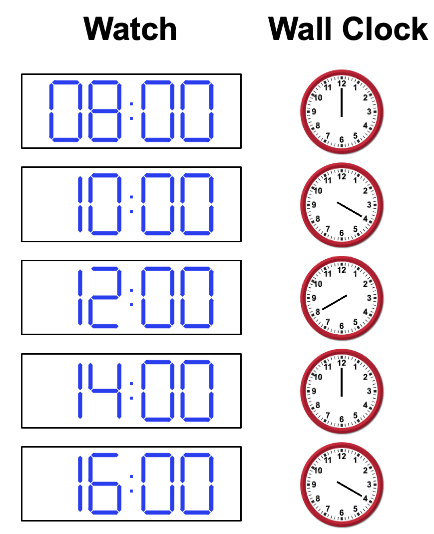
d. Can you tell if the wall clock is running fast or slow?
e. Estimate the frequency of the wall clock (minutes on wall clock per true hours)if you believe it is running fast.
f. Estimate the frequency if you believe it is running slow
g. Are there other frequencies it could be running at?
A post-doc nearby sees what you’re doing, and suggests that maybe you should consider shortening the time on your watch between when you track the wall clock time, and to take the angle relative to the 12 position for better precision. You take the angle every 5 minutes for an hour, and get the following angles (in degrees) of the wall clock:
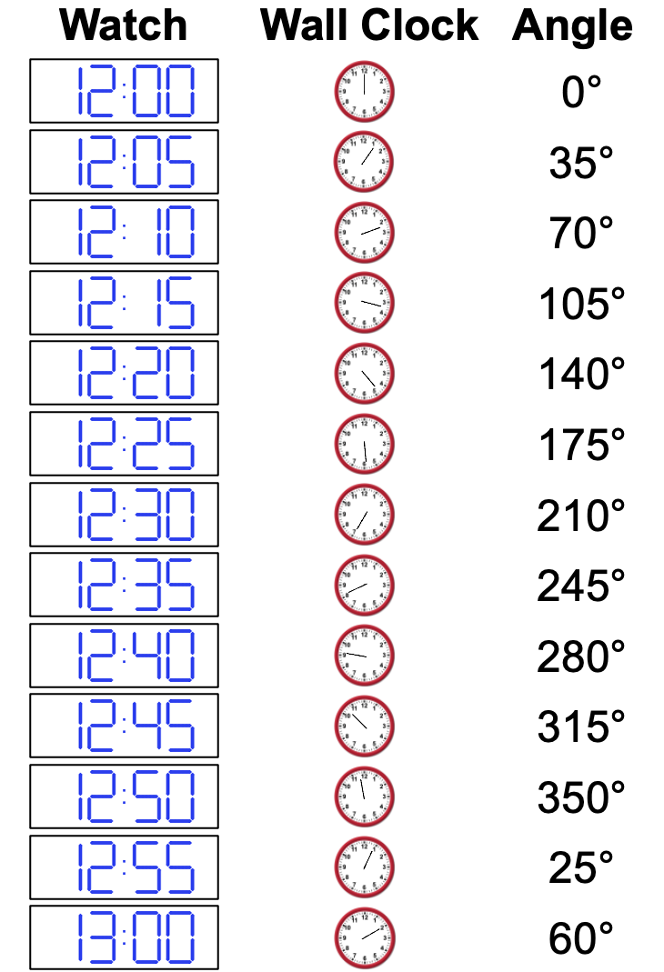
h. Can you tell if the wall clock is running fast or slow?
i. Estimate the frequency of the wall clock in terms of radians per hour.
j. Are you confident in this value? Could it be other frequencies?
- Jezzard, P., & Balaban, R. S. (1995). Correction for geometric distortion in echo planar images from B0 field variations. Magn. Reson. Med., 34(1), 65–73.
- Anzai, Y., Lufkin, R. B., Jabour, B. A., & Hanafee, W. N. (1992). Fat-suppression failure artifacts simulating pathology on frequency-selective fat-suppression MR images of the head and neck. AJNR Am. J. Neuroradiol., 13(3), 879–884.
- Webb, A. G. (2016). Magnetic Resonance Technology: Hardware and System Component Design. Royal Society of Chemistry.
- Schenck, J. F. (1996). The role of magnetic susceptibility in magnetic resonance imaging: MRI magnetic compatibility of the first and second kinds. Med. Phys., 23(6), 815–850.
- Jenkinson, M., Beckmann, C. F., Behrens, T. E. J., Woolrich, M. W., & Smith, S. M. (2012). FSL. Neuroimage, 62(2), 782–790.
- An, H., & Lin, W. (2002). Cerebral oxygen extraction fraction and cerebral venous blood volume measurements using MRI: effects of magnetic field variation. Magn. Reson. Med., 47(5), 958–966.
- Brown, R. W., Cheng, Y.-C. N., Mark Haacke, E., Thompson, M. R., & Venkatesan, R. (2014). Magnetic Resonance Imaging: Physical Principles and Sequence Design. John Wiley & Sons.
- Dietrich, B. E., Brunner, D. O., Wilm, B. J., Barmet, C., Gross, S., Kasper, L., Haeberlin, M., Schmid, T., Vannesjo, S. J., & Pruessmann, K. P. (2016). A field camera for MR sequence monitoring and system analysis. Magn. Reson. Med., 75(4), 1831–1840.
- Frequency drift in MR spectroscopy at 3T. (2021). Neuroimage, 241, 118430.
- El-Sharkawy, A. M., Schär, M., Bottomley, P. A., & Atalar, E. (2006). Monitoring and correcting spatio-temporal variations of the MR scanner’s static magnetic field. MAGMA, 19(5), 223–236.
- de Rochefort, L., Nguyen, T., Brown, R., Spincemaille, P., Choi, G., Weinsaft, J., Prince, M. R., & Wang, Y. (2008). In vivo quantification of contrast agent concentration using the induced magnetic field for time-resolved arterial input function measurement with MRI. Med. Phys., 35(12), 5328–5339.
- Wang, J., Mao, W., Qiu, M., Smith, M. B., & Constable, R. T. (2006). Factors influencing flip angle mapping in MRI: RF pulse shape, slice-select gradients, off-resonance excitation, and B0 inhomogeneities. Magn. Reson. Med., 56(2), 463–468.
- Smith, S. M., Jenkinson, M., Woolrich, M. W., Beckmann, C. F., Behrens, T. E. J., Johansen-Berg, H., Bannister, P. R., De Luca, M., Drobnjak, I., Flitney, D. E., Niazy, R. K., Saunders, J., Vickers, J., Zhang, Y., De Stefano, N., Brady, J. M., & Matthews, P. M. (2004). Advances in functional and structural MR image analysis and implementation as FSL. Neuroimage, 23 Suppl 1, S208-19.
- Alonso-Ortiz, E., Levesque, I. R., Paquin, R., & Pike, G. B. (2017). Field inhomogeneity correction for gradient echo myelin water fraction imaging. Magn. Reson. Med., 78(1), 49–57.
- Akcakaya, M., Doneva, M. I., & Prieto, C. (2022). Magnetic Resonance Image Reconstruction: Theory, Methods, and Applications. Academic Press.