1Introduction
Transmit radiofrequency field mapping (B1+, or B1 for short) is an essential component of quantitative MRI. Accurate knowledge of this field distribution is crucial for multiple applications, including the calibration of quantitative MRI techniques that are sensitive to flip angle inaccuracies, such as variable flip angle T1 mapping Deoni, 2007Boudreau et al., 2017 and quantitative magnetization transfer imaging Ropele et al., 2005Boudreau et al., 2018. Unlike the receive field (B1-), which appears as a simple multiplicative factor that can often be corrected for in post-processing using intensity normalization techniques Sled et al., 1998, the transmit field has a nonlinear impact on MR signal evolution. For example, in spoiled gradient echo sequences, the signal depends on the actual flip angle through complex trigonometric functions in the steady-state signal equation Christensen et al., 1974Fram et al., 1987Gupta, 1977, making it impossible to correct images without detailed knowledge of both the actual flip angles and the specific signal model. B1 maps also play important roles in specific absorption rate calculations Ibrahim et al., 2001, RF coil quality control Yarnykh, 2007, and the study of tissue electrical properties Sled & Pike, 1998Katscher et al., 2009.
This chapter explores several principal methodologies for B1 mapping, each with distinct advantages and practical considerations. The double angle method represents a straightforward magnitude-based approach that acquires images at two different excitation flip angles and computes B1 from their signal ratio Insko & Bolinger, 1993Stollberger & Wach, 1996. While conceptually simple, this technique typically requires long repetition times to minimize T1 dependence, which can limit its time efficiency. In contrast, actual flip-angle imaging (AFI) employs a pulsed steady-state acquisition with two different repetition times, enabling rapid 3D B1 mapping with excellent anatomical coverage in clinically feasible times Yarnykh, 2007. More recently, phase-based methods like the Bloch-Siegert shift technique have emerged that encode B1 information directly into phase signals, offering alternative acquisition strategies Sacolick et al., 2010.
Regardless of the acquisition method, measured B1 maps often require post-processing to address noise, artifacts, and other non-physical variations. Filtering techniques play an important role in producing field maps that better represent the underlying smoothly varying electromagnetic fields while minimizing error propagation to subsequent quantitative MRI applications. Throughout this chapter, we will examine the theoretical foundations, practical implementations, and relative strengths of each B1 mapping approach, providing readers with comprehensive understanding of modern RF field mapping techniques.
2Double Angle techniques
Transmit and Receive RF field amplitudes
In an MRI experiment, magnetic field amplitude of the radiofrequency field (B1) is an an important physical parameter that is a product of the interaction between RF coil design and the subject’s position (volume and relative position to the coil) and physical properties (electromagnetic permittivity ε and permeability μ). In any MRI experiments, two B1 fields appear: the transmit RF field amplitude B1+ and the receive RF field amplitude B1-. The latter, B1-, is often referred to in terms of the receive RF coil sensitivities and this is due to the principle of reciprocity Hoult & Richards, 1976Hoult, 2000 property of RF antennas. In terms of an MRI image, B1- is simply a multiplication factor that varies spatially but doesn’t change between pulse sequences if the subject remains motionless, and techniques to “flatten” images by estimating this field numerically have been developed Sled et al., 1998. Additionally, many quantitative MRI techniques calculate the ratio of images, which eliminates this B1- component from the resulting image.
B1+, however, impacts the resulting MRI images in a much more complex way and is not a simple multiplication factor. B1+ directly perturbs the system of spins by introducing energy in the system, which practically we quantify as the flip angle of an RF pulse. Two different B1+ values will not have the same impact on voxel for different pulse sequences, as spin dynamics and steady-state conditions will vary. For example, let’s say you acquire a saturation recovery image and also a short TR steady-state gradient echo. For an actual flip angle = , the magnetization after TE will be and prior to the RF pulse is given by Eq. 2.5. Thus, not only does B1+ not appear as a simple multiplication factor, a change of B1 will not impact this voxel for both sequences by the same ratio. Thus, knowledge of B1+ through B1 mapping can help us retroactively understand the dynamics of the spins accurately, and can play the role of a calibration factor for many quantitative MRI techniques (e.g. VFA, T2/T2*, qMT, etc). In addition, B1 mapping can also map the electromagnetic properties, but this won’t be discussed in this chapter.
In this chapter, we’ll be discussing a simple but widely used class of methods for B1 mapping, the double angle method. For the sake of simplicity, and for consistency with the quantitative MRI literature, we’ll define B1 = B1+ and will explicitly state B1- when referring to the receive field.
Double Angle method(s)
The Double Angle method (DA or DAM) is a class of B1 mapping techniques where two RF pulses at flip angles α and 2α are applied to a pulse sequence, and the ratio of the images are compared to expected output to produce a B1 map. Several main pulse sequences (Figure 4.1) have been called the double angle method in the literature, and both have their own equations describing the relationship between the expected images and B1. In this chapter, we’ll mostly explore there the α-180 method (Figure 4.1]), and then briefly explain the other method and its similarities/differences.
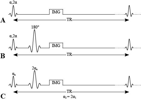
Figure 4.1:Pulse sequences for double angle methods. A) Double angle method using a gradiend echo. B) Double angle method using a 180 degree refocusing pulse. C) Double angle method using a refocusing pulse, acquired with two values and such that .
Gradient echo and 180 degree spin echo methods
This pulse sequence uses a 180 degree spin-echo refocusing pulse and acquires two images using an excitation pulse and . It assumes that there is full signal recovery (long TR), and because it refocuses T2*, it eliminates signal variability caused by B0 in the resulting B1 map Insko & Bolinger, 1993. Alternatively, a gradient echo could be used?
Assuming a refocusing pulse is used (i.e. isn’t dependent on B1), we can develop the equation for a gradient echo and spin echo case.
Thus
and
Using a well known trigonometry identity (see Appendix A for derivation),
We can simplify Eq. 4.5,
And the true flip angle can be calculated from the ratio of these two magnetizations / signals / images:
Knowing that alpha_nominal, B1 is thus:
Figure 4.2:B1 computed from analytical GRE equations for DA sequence
This equation is also used for -180 spin echo pulses, however it assumes no dependency on of the refocusing pulse on B1. Figure 4.3 explores this using Bloch simulations
Figure 4.3:B1 computed from bloch simulations for ideal spin echo and refocusing pulse where FA = 180*B1
Figure 4.4:B1 computed from bloch simulations for spin echo with refocusing pulse where FA = 180*B1, and composite pulse 90x-180y-90x where each 90 and 180 are also multiplied by B1.
3Actual Flip Angle Imaging
Transmit radiofrequency field maps (B1+, or B1 for short) are used in diverse applications in MRI including: the study of electrical properties in tissues in vivo Sled & Pike, 1998Katscher et al., 2009, specific absorption rate (SAR) calculations Ibrahim et al., 2001, the calibration of quantitative T1 Deoni, 2007Boudreau et al., 2017 and T2 Sled & Pike, 2000 maps, better parameter estimation from magnetization transfer measurements Ropele et al., 2005Boudreau et al., 2018, B1 shimming to improve image quality at whole-body ultra high fields Bergen et al., 2007, or quality control of RF coils Yarnykh, 2007. Several B1 mapping techniques have been developed, and they can be broadly divided as magnitude-based and phase-based methods. The double angle method (DAM) is a saturation-recovery magnitude-based method that takes the ratio of the signal intensity of two magnitude images measured with different excitation flip angles Insko & Bolinger, 1993Stollberger & Wach, 1996. The Bloch-Siegert shift technique is a rapid phase-based method that encodes the B1 information into phase signal Sacolick et al., 2010. The actual flip-angle imaging (AFI) is a magnitude-based B1 mapping method that consists of a 3D acquisition that benefits from good anatomical coverage. In addition, this technique allows the acquisitions of whole-body (~7 min) and brain (~3 min) B1 maps leading to a feasible implementation in clinics Yarnykh, 2007. On the other hand, the AFI pulse sequence has certain constraints that need to be considered for this B1 mapping method to be widely deployed. Some of the limitations include the use of spoiler gradients that can give rise to prohibitive SAR values Sacolick et al., 2010, and the pulse sequence modifications on the MRI machine to implement the AFI method.
In this section, we will focus on presenting details about the AFI B1 mapping method. We will cover signal modeling, data fitting, the benefits and the pitfalls of the technique. The figures are generated using the qMRLab module for this method.
Signal Modelling
The pulse sequence of the AFI method (Figure 4.5) is composed of two identical RF pulses and two different delays (TR1 < TR2). After each RF pulse, the signal intensity is acquired followed by a spoiler to destroy the residual transverse magnetization next to the following RF pulse. This method implements a pulsed steady-state signal with a gradient-echo acquisition, thus preventing the use of long repetition times Yarnykh, 2007. It has been demonstrated that if the delays TR1 and TR2 are sufficiently short (e.g. TR1/TR2 = 20 ms/100 ms), and the transverse magnetization is completely spoiled, the ratio of signal intensities (r = S2/S1) depends on the flip angle of applied pulses and is highly insensitive to T1 Yarnykh, 2007.
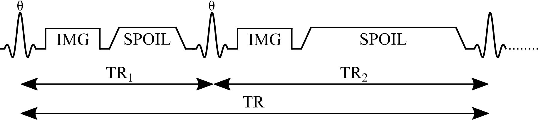
Figure 4.5:Simplified pulse sequence diagram of an actual flip-angle imaging (AFI) pulse sequence with a gradient echo readout. TR1: repetition time 1, TR2: repetition time 2, : excitation flip angle for the measurement, IMG: image acquisition (k-space readout), SPOIL: spoiler gradient.
The magnetization of an AFI experiment can be modeled under steady-state conditions by the implementation of a fast repetition of the sequence (TR1 < TR2 < T1). The solution of the Bloch equations for the AFI method is given by Equations 1 and 2 that represent the longitudinal magnetization before the application of the RF pulses:
Mz1,2 is the longitudinal magnetization of both pulses, M0 is the magnetization at thermal equilibrium, TR1 is the delay time after the first pulse, TR2 is the delay time after the second identical pulse (Figure 4.6), and is the excitation flip angle. The steady-state longitudinal magnetization Mz curves for different T1 values for a range of and TR values are shown in Figure 4.6.
Figure 4.6:Longitudinal magnetization before the first radiofrequency pulse (Eq. 4.10, solid lines) and before the second identical pulse (Eq. 4.11, dashed lines) for three different T1 values.
The analytical solution of the Bloch equations in a steady-state experiment (Eq. 4.10 and Eq. 4.11) makes several assumptions leading to practical challenges. First, it is assumed that the longitudinal magnetization has reached a steady state after a sufficiently large number of repetition times (TR), and that the transverse magnetization is perfectly spoiled prior to each pulse. To explore these properties, a numerical approach known as Bloch simulations is used to estimate the signal from an MRI experiment given a set of sequence parameters. Here, the Bloch simulations allow us to estimate the magnetization using a different number of sequence repetitions, and look at a special case when the steady-state is not achieved (due to a small number of sequence repetitions). As can be seen in Figure 4.7, the number of repetitions required to reach a steady-state depends on T1 and the flip angle.
Figure 4.7:Signal 1 (blue) and Signal 2 (red) curves simulated using Bloch simulations (solid lines) for a number of repetitions ranging from 1 to 150, plotted against the ideal case (Eq. 4.10 and Eq. 4.11 – dashed lines). Simulation details: TR1 = 20 ms, TR2 = 100 ms, T1 = 900 ms, 100 spins. Ideal spoiling was used for this set of Bloch simulations (transverse magnetization was set to 0 at the end of each TR1,2).
In practice, gradient and RF spoiling are important parameters to consider in an AFI experiment. A combination of both Zur et al., 1991Bernstein et al., 2004 is typically recommended, and Figure 4.8 shows how this better approximates the ideal spoiling case.
Figure 4.8:Signal 1 curves estimated using Bloch simulations for three categories of signal spoiling: (1) ideal spoiling (blue), gradient & RF Spoiling (red), and no spoiling (orange). Simulation details: TR1 = 20 ms, TR2 = 100 ms, T1 = 900 ms, T2 = 100 ms, TE = 5 ms, 100 spins. For the ideal spoiling case, the transverse magnetization is set to zero at the end of each TR. For the gradient & RF spoiling case, each spin is rotated by different increments of phase (2𝜋 / # of spins) to simulate complete dephasing from gradient spoiling, and the RF phase of the excitation pulse is Bernstein et al., 2004 with Zur et al., 1991 after each TR.
Data Fitting
The ratio of Eq. 4.10 and Eq. 4.11, gives rise to Eq. 4.12 that depends on the parameters T1, TR1, TR2 and the excitation flip angle ().
Eq. 4.12 can be simplified if the Taylor series expansion of the exponential function is used, followed by a first-order approximation to its terms. For this expansion, short TR1 and TR2 (TR1 < T1 and TR2 < T1) are assumed to approximate the signal intensities ratio (Eq. 4.13) where n = TR2/TR1.
Finally, a measure of the actual flip-angle () can be achieved by solving Eq. 4.13 to obtain Eq. 4.14, which only depends on the signal intensities ratio (r = S2/S1) and the parameters TR1 and TR2.
The actual flip-angle is estimated using an approximation (Eq. 4.13) of a complete analytical solution (Eq. 4.12), and the nature of this approximation makes it worthwhile to assess the accuracy of the signal intensities ratio between both equations. Next, a set of simulations are displayed to analyze how the choice of r is affected by T1, TR1 and TR2. First, the effect of the relaxation time T1 is simulated in Figure 4.9 for both the approximation and the complete analytical solution.
Figure 4.9:Effect of the relaxation time T1 on the ratio r. Signal intensities ratio is plotted as a function of the flip angle for the complete analytical solution (Eq. 4.12 - blue) and the first-order approximation (Eq. 4.13 - orange). AFI simulation details: TR1 = 20 ms, TR2 = 100 ms and variable T1.
The signal ratio r is highly insensitive to the relaxation time T1, except for the low T1 values and large flip angles (>70°). This shows that the Taylor expansion is a good approximation to the signal ratio r because it is possible to get rid of the inverse quadratic T1 dependance by taking the first-order terms of the expansion.
The effect of the TR1 parameter on the signal ratio is shown in Figure 4.10. To assess the influence of the repetition time, we fix n=5 and vary the parameter TR1 in accordance to the relation n = TR2/TR1. As TR1 increases (> 50 ms), the approximated ratio r slightly deviates from the analytical approach. Although the deviation is slight only at high flip angles, a good signal ratio approximation can be achieved for a wide range of flip angles and repetition times.
Figure 4.10:Effect of the repetition time TR1 on the ratio r. Signal intensities ratio is plotted as a function of the flip angle for the complete analytical solution (Eq. 4.12 - blue) and the first-order approximation (Eq. 4.13 - orange). AFI simulation details: Variable TR1 ranging from 10 to 60 ms, fixed ratio n = 5 and T1 = 900 ms.
Finally, the effect of the parameter n on the signal ratio r (Figure 4.11) does not seem to significantly affect the signal ratio between the approximated equation and the analytical approach. However, the parameter n has a major impact on the sensitivity of the AFI method to variations in the flip angle. Figure 4.11 shows that the increase of the parameter n (= TR2/TR1) allows for improvement of the dynamic range of flip angles measurements. These simulations have shown that an optimal implementation of the AFI method requires a careful selection of sequence parameters.
Figure 4.11:Effect of n (TR2 to TR1 ratio) on the ratio r. The signal intensities ratio is plotted as a function of the flip angle for the complete analytical solution (Eq. 4.12 - blue) and the first-order approximation (Eq. 4.13 - orange). AFI simulation details: Variable n ranging from 2 to 6, fixed TR1 = 20 ms and T1 = 900 ms.
Figure 4.12 displays an example AFI dataset and its corresponding field B1 map in a healthy human brain. Although not clearly visible, both AFI images present a small Gibbs ringing artifact that is propagated and amplified due to the AFI calculation consisting of the division of both images Boudreau et al., 2017. The ringing artifact is clearly seen in the unfiltered/raw B1 field map shown in Figure 4.12 (right).
Figure 4.12:Example actual flip-angle imaging dataset (left) and a resulting raw B1 map of a healthy adult brain (right). The relevant VFA protocol parameters used were: TR1 = 20 ms, TR2 = 100 ms and = 60°. The B1 map (right) was fitted using the approximate r ratio (Eq. 4.14).
The ringing artifact shown in Figure 4.12 can be attenuated by implementing a smoothing process. Figure 4.13 shows the raw (left) and the filtered (right) B1 map where a median filter was used to smooth the field map.
Figure 4.13:Raw (left) and filtered (right) B1 map. A median filter of size 7x7x7 pixels was used to attenuate the Gibbs ringing artifact.
Benefits and Pitfalls
B1 mapping is of interest for diverse MRI applications, and several mapping techniques have been developed. The DAM method consists of acquiring two scans at two different flip angles. To avoid the dependence of the signal on T1, long repetition times are required to allow the recovery of the longitudinal magnetization between pulses Yarnykh, 2007Insko & Bolinger, 1993. The AFI method overcomes this practical limitation by repeating the pulse sequence at a fast rate to achieve a pulsed state of magnetization and shorter time delays between pulses. In addition, due to scan-time constraints, B1 mapping methods are often implemented in 2D Chavez & Stanisz, 2012. However, the accuracy of the measurements of 2D B1 mapping techniques is compromised by the slice profile effects due to the problem of nonuniform excitation across slices Yarnykh, 2007Chavez & Stanisz, 2012. The AFI method on the other hand, adresses this issue using a fast 3D implementation leading to scans with an excellent anatomical coverage in clinically feasible times, with an increase in signal-to-noise ratio compared to 2D multislice acquisitions.
The performance of the AFI method is based on the following assumptions. First, the two images acquired at different times should be registered to avoid motion effects. It is also assumed that the signal is insensitive to the main magnetic field non-uniformities and chemical shift effects that are canceled out when taking the signal ratio r Yarnykh, 2007. Despite some clear advantages over other B1 mapping techniques, the application of spoiler gradients to mitigate the T1 dependence can be a limitation due to significant levels of RF power depositions Sacolick et al., 2010. Furthermore, it is necessary to adapt the AFI pulse sequence to different scanner manufacturers, and programming experience is required to bring this technique into the clinic.
4Filtering
The behaviour of electromagnetic fields produced by RF antennas are bound by the laws of physics. The Maxwell equations impose many limitations on how these fields can not only vary spatially and temporally, but how the electric and magnetic fields are linked. While propagating magnetic fields interface of boundary between materials can be discontinuous (a result of Maxwell’s equations), it’s been shown in the context of MRI and tissues that the magnetic field amplitudes are expected to be smoothly varying when using clinical MRIs Sled & Pike, 1998Sled et al., 1998. At ultra-high fields, standing wave artifacts can lead to more B1 variations and even signal nulls, however the field amplitude nonetheless varies continuously Uğurbil, 2018Vaughan et al., 2001Yang et al., 2002. Thus, for both B1+ and B1-, their amplitude is expected to be a smoothly varying multiplicative field, and at clinical field strength it’s also expected to be a slowly or low frequency varying field.
In practice, measured B1+ maps are rarely perfectly smooth over the anatomy-of-interest being imaged. Figure 4.14 shows a comparison of measured B1 maps in the brain produced by three methods: double angle, actual flip angle imaging (AFI), and Bloch-Siegert shift.
Figure 4.14:Example B1 maps (right column) along with their raw acquired data (left and middle columns) for three different B1 mapping techniques: double angle (top row), actual flip angle imaging (AFI; middle row), and Bloch-Siegert shift (bottom row).
The overall “shape” of the B1 map is the same for all three maps, and this nonuniformity pattern is expected due to the elliptical shape of the brain and its electromagnetic properties Sled & Pike, 1998. We see in the B1 maps of Figure 4.14 that there is some noise, some distinguishable anatomical structures (caused by T1 sensitivity and/or k-space propagation susceptibility effects), and in one case (AFI) an artifact caused by Gibbs ringing in the acquired images. All of these variations are not present in the actual B1+ field that the spins experience during a pulse sequence, and so using this “raw” B1 map to calibration flip angles or RF power for other quantitative MRI techniques (eg. variable flip angle T1 mapping, quantitative magnetization transfer) risks introducing errors during the correction.
Although not a perfect solution, researchers often smoothen their B1 maps Yarnykh, 2007Lutti et al., 2010Boudreau et al., 2017 in an effort to mitigate the error propagation from the B1+ map noise and artifacts prior to use for other techniques. This chapter will discuss some common ways this B1 map smoothing is achieved, show some examples of their benefits and weaknesses, and discuss some best practices.
Filters and smoothing
There are two main ways that field maps are smoothened in practice: filters and fitting. The study of filters is typically presented in a signal processing context, however its basic principles (in particular, convolutions) are observed in many other fields of study, in particular physics.
We’ll begin by providing a very brief overview of some key filtering properties, then move on to some illustrative 1D examples related to MRI situations before finally returning to their applications in actual B1 maps.
Filtering is presented as a convolution process to produce an output that is smoother, meaning less sharp edges. A convolution is the multiplication of a kernel (a predetermined function or property, such as the mean, median, Gaussian function, etc) that is shifted at each point of the signal or image, and the summed value of this multiplication is assigned to the time or spatial point where it was applied. Figure 4.16 illustrates this for the mean using a three-position mean as a kernel:
In the context of MRI, the mean is not the best choice for a filter, as it is sensitive to high values relative to the base signal. The median is a better choice, which we’ll demonstrate in the next section. In terms of equations, the convolution is shown using the symbol , such that analytically it is represented as:
where is the signal of interest and is the kernel. Not every kernel will lead to smoothing (reduction of high frequencies) of the signal of interest when convolved, however the Gaussian distribution is one such smoothing function:
where is the center position of the distribution, and is a measure of the width. The convolution using this function with a 9-point sample for different widths is shown in Figure 4.16.
Figure 4.16:Convolution using a Gaussian kernel
One property of the convolution is that the convolution of two functions is the multiplication of the Fourier transforms of each function following by an inverse Fourier transform:
Although convolutions can be computed this way and may me more conceptually clear, particularly the role of the kernel, practically this ends up being slower than the convolution method when using only a small number of samples for the kernel.
As for “smoothing” the signal using fitting, splines are simply a piecewise fit of your signal to some function with a continuity condition set at different points throughout the signal. Typically this is done using polynomials, such as a third-order polynomial: . There are a lot of different algorithms and ways to do this, which is out of scope for this work.
B1 map examples
Let’s revisit our initial B1 maps in Figure 4.14 and see how they respond to the filters we’ve explored in the previous section. The double angle B1 maps were mostly impacted by noise and structural T1 patterns, AFI had some artifacts that were caused by Gibbs ringing in the raw images, and the Bloch-Siegert B1 map had an artifact caused by a phase pole at the end of a fringe line. Figure 4.22 shows each of the B1 map and the filtered maps using the median, Gaussian, and spline filtering techniques.
Figure 4.22:Filtered B1 maps
All three methods worked well with the double angle B1 map, and the outputs of the median and Gaussian are most similar. The top right corner of the spline-filtered double angle B1 map has higher intensity, likely due to an edge effect as discussed in the 1D example section. For AFI, median and gaussian filters removed most of the repeated variations, whereas spline-filtering didn’t at the medium filter strength. Lastly, for Bloch-Siegert, the median filter performed well at removing the noise and smoothing out the artifact, though some still remains. For the Gaussian and spline cases, there was a single pixel in the left that had very high value in the unfiltered images and this led to a spreading of high B1 values to nearby voxels, something that didn’t occur for the median filter case. If either of these filters were used in an automated pipeline without quality control, inaccurate B1 values would have been spread, which is undesireable.
Recommendations, benefits, and pitfalls
Overall, median, Gaussian, and spline filters perform at smoothing noisy B1 maps. If image artifacts exists in the B1 maps, then the choice of filter could impact the output B1 map. In all our B1 map examples (Figure 4.22), a 5x5 voxel median filter would have performed sufficiently all while avoiding spreading errors. This may be a relatively safe filter to try first for clinical use in the brain at clinical field strengths. In other field strengths or anatomies, or if different artifacts exist, this may not always be the case. Good care should always be applied when selecting a filter; know why you are using it, what its potential drawbacks are, and look for error spreading in the output B1 map.
If your filtered B1 map is intended for use at boundary edges, such as grey matter, extra precautions should be taken when applying filters and doing quality control. Know how your filters handle edges, and if needed choose to mirror or extrapolate B1 values beyond the masked region of interest. Quality control is important, as there can be substantial edge artifacts when using filters.
Finally, remember that using the unfiltered B1 map is also a choice, and many researchers use these. It’s important to report if you filtered or not your B1 maps when reporting them in your research.
5Appendix A
6Exercises
- Deoni, S. C. L. (2007). High-resolution T1 mapping of the brain at 3T with driven equilibrium single pulse observation of T1 with high-speed incorporation of RF field inhomogeneities (DESPOT1-HIFI). J. Magn. Reson. Imaging, 26(4), 1106–1111.
- Boudreau, M., Tardif, C. L., Stikov, N., Sled, J. G., Lee, W., & Pike, G. B. (2017). B1 mapping for bias-correction in quantitative T1 imaging of the brain at 3T using standard pulse sequences. J. Magn. Reson. Imaging, 46(6), 1673–1682.
- Ropele, S., Filippi, M., Valsasina, P., Korteweg, T., Barkhof, F., Tofts, P. S., Samson, R., Miller, D. H., & Fazekas, F. (2005). Assessment and correction of B1-induced errors in magnetization transfer ratio measurements. Magn. Reson. Med., 53(1), 134–140.
- Boudreau, M., Stikov, N., & Pike, G. B. (2018). B1 -sensitivity analysis of quantitative magnetization transfer imaging. Magn. Reson. Med., 79(1), 276–285.
- Sled, J. G., Zijdenbos, A. P., & Evans, A. C. (1998). A nonparametric method for automatic correction of intensity nonuniformity in MRI data. IEEE Trans. Med. Imaging, 17(1), 87–97.
- Christensen, K. A., Grant, D. M., Schulman, E. M., & Walling, C. (1974). Optimal determination of relaxation times of Fourier transform nuclear magnetic resonance. Determination of spin-lattice relaxation times in chemically polarized species. The Journal of Physical Chemistry, 78(19), 1971–1977. 10.1021/j100612a022
- Fram, E. K., Herfkens, R. J., Johnson, G. A., Glover, G. H., Karis, J. P., Shimakawa, A., Perkins, T. G., & Pelc, N. J. (1987). Rapid calculation of T1 using variable flip angle gradient refocused imaging. Magnetic Resonance Imaging, 5(3), 201–208. 10.1016/0730-725x(87)90021-x
- Gupta, R. K. (1977). A new look at the method of variable nutation angle for the measurement of spin-lattice relaxation times using fourier transform NMR. Journal of Magnetic Resonance (1969), 25(1), 231–235. 10.1016/0022-2364(77)90138-x
- Ibrahim, T. S., Lee, R., Baertlein, B. A., & Robitaille, P.-M. L. (2001). B1 field homogeneity and SAR calculations for the birdcage coil. Phys. Med. Biol., 46, 609–619.
- Yarnykh, V. L. (2007). Actual flip-angle imaging in the pulsed steady state: a method for rapid three-dimensional mapping of the transmitted radiofrequency field. Magn. Reson. Med., 57(1), 192–200.
- Sled, J. G., & Pike, G. B. (1998). Standing-wave and RF penetration artifacts caused by elliptic geometry: an electrodynamic analysis of MRI. IEEE Trans. Med. Imaging, 17(4), 653–662.
- Katscher, U., Voigt, T., Findeklee, C., Vernickel, P., Nehrke, K., & Dössel, O. (2009). Determination of electric conductivity and local SAR via B1 mapping. IEEE Trans. Med. Imaging, 28(9), 1365–1374.
- Insko, E. K., & Bolinger, L. (1993). Mapping of the radiofrequency field. J. Magn. Reson. A, 103(1), 82–85.
- Stollberger, R., & Wach, P. (1996). Imaging of the active B1 field in vivo. Magn. Reson. Med., 35(2), 246–251.
- Sacolick, L. I., Wiesinger, F., Hancu, I., & Vogel, M. W. (2010). B1 mapping by Bloch-Siegert shift. Magn. Reson. Med., 63(5), 1315–1322.