1Introduction
T2 relaxation, also known as the transverse or spin-spin relaxation, is characterized by the dephasing of spins, leading to a reduction of the total magnetization in the x-y plane. In practical terms, the T2 value represents the upper limit of the signal decay time under ideal imaging conditions. In practice, magnetic field inhomogeneities cause the transverse magnetization to decay faster than what is captured by T2 relaxation. These inhomogeneities can be macroscopic, caused by factors such as metallic implants or air-tissue interfaces, or microscopic, resulting from differences in magnetic susceptibility between tissues Chavhan et al., 2009Cohen-Adad, 2014 . When considering this phenomenon, we refer to the transverse relaxation as T2*.
T2 mapping, a quantitative magnetic resonance imaging method, offers images of T2 relaxation times (called T2 maps) providing valuable insights into tissue composition. Given that T2 relaxation is sensitive to specific microstructural changes associated with diseases, such as iron accumulation, myelination and inflammation Dortch, 2020, it is considered a promising modality for clinical and research applications. Commonly used T2-mapping techniques are split into two categories: the mono-exponential methods, which consider that the voxel’s signal arises from a single tissue compartment, and multi-exponential methods, where various tissues that contribute to a single voxel’s signal are considered. Recently, novel techniques for T2 mapping have emerged beyond the conventional techniques that were developed for NMR, such as MR fingerprinting (Ma et al., 2013), a fast relaxation mapping technique that uses a single image acquisition to quantify multiple parameters Hamilton et al., 2017.
In the following sections, we will introduce the current state-of-the-art signal modeling and data fitting theory for both mono-exponential and multi-exponential T2 mapping, as well as the benefits and pitfalls of both approaches. An overview of some common applications of T2 mapping (e.g., myelin water fraction (MWF) imaging) will also be presented. We will also cover the fundamentals of T2* mapping and explore how its signal decay curve can differ from that of T2 relaxation.
T2 mapping vs T2-weighted imaging
The standard practice in clinical MRI is T2-weighted imaging (T2w), i.e. images in which the different tissues produce signals according to their T2 relaxation times. T2w images are considered qualitative, as they rely on differences in T2 relaxation of various tissues to provide contrast rather than actual quantitative tissue measurements, thus making their interpretation dependent on the observer. Meanwhile, T2 mapping is considered a quantitative technique, as it directly measures the T2 relaxation time of tissues by fitting multiple data points to a decay curve to calculate the T2 constant. The objective nature of T2 mapping makes it a promising technique for various applications in both clinical practice and research, including disease progression monitoring and the identification of novel biomarkers. Another advantage of T2 mapping is that it allows for consistent comparisons across different imaging protocols, thereby enhancing reproducibility and making it ideal for longitudinal and multi-institutional studies Cheng et al., 2012. Figure 3.1 shows several examples of T2w images acquired at different echo times, compared to the T2 map generated by fitting the decay curve.
Figure 3.1:T2-weighted images at different TE, compared to T2 map following data fitting of the T2 decay curve.
Click here to view the qMRLab (MATLAB/Octave) code that generated Figure 3.1.
%% Requirements
% qMRLab must be installed: git clone https://www.github.com/qMRLab/qMRLab.git
% The mooc chapter branch must be checked out: git checkout mooc-03-T2
% qMRLab must be added to the path inside the MATLAB session: startup

% Define the model
Model = mono_t2;

% Load data into environment, and rotate mask to be aligned with IR data
data = struct;
data.SEdata = double(load_nii_data('../data/mono_t2/SEdata.nii.gz'));
data.Mask = double(load_nii_data('../data/mono_t2/Mask.nii.gz'));

% Define fitting parameters
EchoTime  = [12.8000; 25.6000; 38.4000; 51.2000; 64.0000; 76.8000; 89.6000; 102.4000; 115.2000; 128.0000; 140.8000; 153.6000; 166.4000; 179.2000; 192.0000; 204.8000; 217.6000; 230.4000; 243.2000; 256.0000; 268.8000; 281.6000; 294.4000; 307.2000; 320.0000; 332.8000; 345.6000; 358.4000; 371.2000; 384.0000];
Model.Prot.SEdata.Mat = [ EchoTime ];
FitResults = FitData(data,Model,0);

% T2w MRI data at different TE values
TE_1 = imrotate(squeeze(data.SEdata(:,:,:,1).*data.Mask),-90);
TE_2 = imrotate(squeeze(data.SEdata(:,:,:,10).*data.Mask),-90);
TE_3 = imrotate(squeeze(data.SEdata(:,:,:,20).*data.Mask),-90);
TE_4 = imrotate(squeeze(data.SEdata(:,:,:,30).*data.Mask),-90);

% Extract the T2 map from FitResults and rotate it
T2_map = imrotate(squeeze(FitResults.T2.*data.Mask), -90);

% Plotting the images
figure;

subplot(2, 3, 1);
imagesc(TE_1);
colormap(gray);
colorbar;
axis image;
title('TE = 12.80 ms');
xlabel('X-axis');
ylabel('Y-axis');
caxis([0, 2500]);

subplot(2, 3, 2);
imagesc(TE_2);
colormap(gray);
colorbar;
axis image;
title('TE = 128.00 ms');
xlabel('X-axis');
ylabel('Y-axis');
caxis([0, 2500]);

subplot(2, 3, 3);
imagesc(TE_3);
colormap(gray);
colorbar;
axis image;
title('TE = 256.00 ms');
xlabel('X-axis');
ylabel('Y-axis');
caxis([0, 2500]);

subplot(2, 3, 4);
imagesc(TE_4);
T2_map = imrotate(squeeze(FitResults.T2.*data.Mask),-90);
colormap(gray);
colorbar;
axis image;
title('TE = 384.00 ms');
xlabel('X-axis');
ylabel('Y-axis');
caxis([0, 2500]);

subplot(2, 3, 5);
imagesc(T2_map);
colormap(gray);
colorbar;
axis image;
title('T2 map');
xlabel('X-axis');
ylabel('Y-axis');
caxis([80, 150]);

%% Export

EchoTimes = [EchoTime(1), EchoTime(10), EchoTime(20), EchoTime(30)]
save("T2w_vs_T2map.mat", "T2_map", "TE_1", "TE_2", "TE_3", "TE_4", "EchoTimes")2Monoexponential T2 Mapping
The simplest technique for performing T2-mapping involves the acquisition of multiple images using a single-echo sequence with different echo times (TE). This set of data can then be used to fit the T2 from the decaying signal curve Milford et al., 2015. However, this method is typically not employed in-vivo due to its prohibitively long acquisition times.
Multi-spin echo (MSE) sequences, based on the Carr-Purcell-Meiboom-Gill (CPMG) pulse train Carr & Purcell, 1954Meiboom & Gill, 1958, employ multiple 180-degree refocusing pulses to generate multiple echoes within a single acquisition (Figure 3.2) Fatemi et al., 2020Milford et al., 2015. This substantially reduces the scan time relative to acquiring multiple echoes using separate single-SE acquisitions, making MSE the sequence of choice in clinical settings.
The original Carr-Purcell method, which involves applying a 90-degree pulse followed by a series of 180-degree pulses along the same axis (e.g., x-axis), was designed to mitigate diffusion effects by preventing phase accumulation. However, this approach can lead to the accumulation of imperfections in the 180-degree pulses, resulting in a faster than expected loss of transverse magnetization (Mxy) and inaccurate T2 measurements Brown et al., 2014. The Meiboom-Gill improvement addresses this issue by applying the initial 90-degree pulse along one axis (e.g., x-axis) and the subsequent 180-degree pulses along a perpendicular axis (e.g., y-axis). This phase cycling distributes errors such that they average out over time, producing a more stable and accurate echo train Brown et al., 2014.
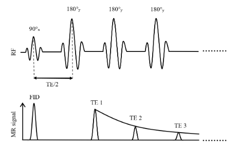
Figure 3.2:Simplified illustration of a multi-spin echo sequence for T2 mapping based on the Carr-Purcell-Meiboom-Gill method
To fit the data using the mono-exponential model, homogeneity within each voxel is assumed implicitly, implying a consistent T2 decay time across the tissue. This results in a single fitted T2 value for each voxel in the image. Although it is widely used, the mono-exponential model has been shown to be insufficient for proper estimation of tissue T2 relaxation times, given that the signal in a voxel often arises from multiple tissue components with different T2 values Graham et al., 1996. In a later section of this chapter, we will cover the multi-exponential method and discuss its use in applications such as myelin water fraction (MWF) imaging.
Signal Modelling
The decay of the transverse magnetization (Mxy) is exponential and can be derived from the transverse component of the Bloch equations:
where Mz(0-) is the longitudinal magnetization immediately preceding the 90 degree excitation pulse. By using this equation, we make the assumption that the measured signal is proportional to the transverse magnetization (Mxy), and that Mz(0-) remains constant regardless of echo time (TE) Dortch, 2020.
Figure 3.3 shows transverse relaxation curves for T2 and T2* values for white matter and gray matter, using the relaxation times from Siemonsen et al., 2008.
Figure 3.3:Transverse relaxation decay curves for T2 and T2* values in white matter and gray matter. The T2 and T2* constants were taken from Siemonsen et al., 2008.
In NMR physics, it has been shown that T2 relaxation times must be equal to or shorter than 2 T1 Levitt, 2008; however, it has been demonstrated that T2 can exceed T1 in very rare cases Traficante, 1991. In living organisms however, T2 is always shorter than T1.
Click here to view the qMRLab (MATLAB/Octave) code that generated Figure 3.3.
%% Requirements
% qMRLab must be installed: git clone https://www.github.com/qMRLab/qMRLab.git
% The mooc chapter branch must be checked out: git checkout mooc-03-T2
% qMRLab must be added to the path inside the MATLAB session: startup

%% T2 and T2* decay curves
% Script to display T2 and T2* relaxometry curves for different tissues

% Simulation parameters
params.TE = linspace(0, 300, 100); % Echo times (in ms)

% Define T2 values for different tissues
params.T2_WM = 109.77; % T2 of white matter (in ms)
params.T2_GM = 96.07; % T2 of gray matter (in ms)

% Define T2* values for different tissues
params.T2star_WM = 67.63; % T2* of white matter (in ms)
params.T2star_GM = 48.48; % T2* of gray matter (in ms)

% Generate T2 and T2* decay signals
signal_WM_T2 = exp(-params.TE / params.T2_WM);
signal_GM_T2 = exp(-params.TE / params.T2_GM);
signal_WM_T2star = exp(-params.TE / params.T2star_WM);
signal_GM_T2star = exp(-params.TE / params.T2star_GM);

% Plot the T2 and T2* signals
figure;
hold on;
plot(params.TE, signal_WM_T2, '-b', 'DisplayName', 'T2 = 109.77 ms (white matter)');
plot(params.TE, signal_GM_T2, '-r', 'DisplayName', 'T2 = 96.07 ms (gray matter)');
plot(params.TE, signal_WM_T2star, '--b', 'DisplayName', 'T2* = 67.63 ms (white matter)');
plot(params.TE, signal_GM_T2star, '--r', 'DisplayName', 'T2* = 48.48 ms (gray matter)');
xlabel('Echo Time - TE (ms)');
ylabel('Transverse Magnetization (Mxy)');
legend();
title('T2 and T2* Decay Signals');

%% Export

TE = squeeze(params.TE)
save("t2_and_t2star_curvs.mat", "signal_WM_T2", "signal_GM_T2", "signal_WM_T2star", "signal_GM_T2star", "params")
Data Fitting
The T2 signal decay for the mono-exponential model is described mathematically as :
where S0 is the signal intensity immediately following the excitation pulse Dortch, 2020Milford et al., 2015.
In practice, B1 inhomogeneities and RF pulse imperfections can influence the T2 signal decay curve and result in inaccurate T2 estimations. This may cause refocusing pulses to deviate from the ideal 180 degrees, generating additional echoes known as stimulated or spurious echoes. These unwanted echoes can contaminate the signal decay, resulting in erroneous T2 estimations McPhee & Wilman, 2018. To account for these stimulated echoes, some studies have shown that T2 fitting accuracy can be improved either by using only even-numbered echoes Focke et al., 2011Kim et al., 2009, or by discarding the first echo Biasiolli et al., 2013Milford et al., 2015.
2.1T2*
Until now, we have assumed that the transverse signal (Mxy) decays exponentially with the echo time divided by the T2 constant (see Eq. 3.3). However, in practice, other factors such as B0 inhomogeneities can cause a more rapid loss of the transverse signal; this results in a faster transverse decay, which is referred to as T2* relaxation (see Figure 3.1).
The relation between T2 and T2* is described as follows Brown et al., 2014:
Where T2′ quantifies the portion of relaxation which is due to magnetic field inhomogeneities. Some studies suggest that T2′ mapping, which can be performed by removing the T2 relaxation effect from T2*, could offer valuable insights for brain disease diagnosis, notably by quantifying blood oxygenation levels Lee et al., 2014 and to predict infarct growth in acute stroke patients Siemonsen et al., 2008.
The T2* decay can then be calculated using the same methods as T2, where Eq. 3.3 can be rewritten as follows :
Unlike T2 mapping, which uses spin echo type sequences, T2* mapping is performed using gradient echo sequences (GRE), as they are sensitive to magnetic field inhomogeneities Cohen-Adad, 2014Markl & Leupold, 2012. Nonetheless, there are specialized sequences such as the spin and gradient echo (SAGE) sequence Stokes et al., 2014 that enable the simultaneous acquisition of both T2 and T2*.
2.2Noise
In MRI, noise in the data can make it harder to accurately fit the T2 decay curve, which is problematic given the necessity for highly precise T2 values in clinical contexts. This issue is particularly pronounced when using pixel-wise T2 mapping, as the signal-to-noise (SNR) is much lower compared to region-of-interest (ROI) T2 mapping approaches Sandino et al., 2015. Figure 3.4 shows how varying the level of noise in the acquired data can influence the fitting of the T2 relaxation curve and the resulting T2 constant. As observed in this figure, a low SNR can have a considerable impact on the T2 fitting process.
Figure 3.4:Impact of noise on T2 relaxometry fitting. The figure shows a single voxel fit with a true T2 relaxation time of 109 ms. As the noise level increases, the accuracy of the T2 fitting decreases, leading to deviations in the estimated T2 relaxation time from the true value. This demonstrates how higher noise levels can adversely affect the reliability of T2 measurements and may result in inaccurate representations of tissue relaxation properties.
The number of echoes used in T2 relaxometry is influenced by several factors, including the need for adequate spacing between echoes, the potential risk of heating the sample, and the challenges associated with processing data from samples with low signal-to-noise ratios. Therefore, selecting an optimal number of echoes is crucial for achieving accurate and reliable results while addressing these constraints Shrager et al., 1998. The Cramer-Rao lower-bound (CRLB) method is a statistical tool that can be used in the context of T2 relaxometry to estimate the smallest possible variance, known as the lower bound, of an unbiased estimator given the noise present in the data Cavassila et al., 2001. Using the lower bounds, the optimal number of echoes needed to accurately fit the T2 decay curve can be determined, ensuring more robust T2 mapping Jones et al., 1996. In their work, Shrager et al., 1998 introduced another method for optimizing the selection of echo time points to improve the accuracy of T2 value estimates based on a predetermined range of expected T2 values. Their approach demonstrated superior accuracy compared to conventional methods that use uniformly-spaced echo times, suggesting that these methods are not optimal for T2 curve fitting accuracy.
Click here to view the qMRLab (MATLAB/Octave) code that generated Figure 3.5.
%% Requirements
% qMRLab must be installed: git clone https://www.github.com/qMRLab/qMRLab.git
% The mooc chapter branch must be checked out: git checkout mooc-03-T2
% qMRLab must be added to the path inside the MATLAB session: startup
%% T2 and T2* decay curves

close all
clear all
clc

% Define model
Model = mono_t2;

params.TE = linspace(0, 300, 100); % Echo times (in ms)

% Define signal parameters for different tissues
x = struct;
x.M0 = 1000;
x.T2 = 109; % (in ms)

% Define the signal-to-noise ratio
Opt1.SNR = 10;
Opt2.SNR = 50;
Opt3.SNR = 90;
Opt4.SNR = 130;

% Run the simulation for T2 and T2* decay curves
[FitResult_SNR10, data_SNR10] = Model.Sim_Single_Voxel_Curve(x, Opt1);
[FitResult_SNR50, data_SNR50] = Model.Sim_Single_Voxel_Curve(x, Opt2);
[FitResult_SNR90, data_SNR90] = Model.Sim_Single_Voxel_Curve(x, Opt3);
[FitResult_SNR130, data_SNR130] = Model.Sim_Single_Voxel_Curve(x, Opt4);

% T2 constants
T2_SNR10 = FitResult_SNR10.T2;
T2_SNR50 = FitResult_SNR50.T2;
T2_SNR90 = FitResult_SNR90.T2;
T2_SNR130 = FitResult_SNR130.T2;

% T2 decay curves
signal_SNR10 = FitResult_SNR10.M0/1000 * exp(-params.TE / FitResult_SNR10.T2);
signal_SNR50 = FitResult_SNR50.M0/1000 * exp(-params.TE / FitResult_SNR50.T2);
signal_SNR90 = FitResult_SNR90.M0/1000 * exp(-params.TE / FitResult_SNR90.T2);
signal_SNR130 = FitResult_SNR130.M0/1000 * exp(-params.TE / FitResult_SNR130.T2);

% Noisy data points
EchoTimes  = [12.8000; 25.6000; 38.4000; 51.2000; 64.0000; 76.8000; 89.6000; 102.4000; 115.2000; 128.0000; 140.8000; 153.6000; 166.4000; 179.2000; 192.0000; 204.8000; 217.6000; 230.4000; 243.2000; 256.0000; 268.8000; 281.6000; 294.4000; 307.2000; 320.0000; 332.8000; 345.6000; 358.4000; 371.2000; 384.0000];
SEdata_SNR10 = data_SNR10.SEdata/1000;
SEdata_SNR50 = data_SNR50.SEdata/1000;
SEdata_SNR90 = data_SNR90.SEdata/1000;
SEdata_SNR130 = data_SNR130.SEdata/1000;

%% Export

disp(EchoTimes)
disp(params.TE)

save("t2_noise_simulation.mat", "params", "signal_SNR10", "signal_SNR50", "signal_SNR90", "signal_SNR130", "T2_SNR10", "T2_SNR50", "T2_SNR90", "T2_SNR130", "SEdata_SNR10", "SEdata_SNR50", "SEdata_SNR90", "SEdata_SNR130", "EchoTimes")
Benefits and Pitfalls
The main benefit of mono-exponential T2 mapping is its simplicity and straightforward implementation, making it a convenient and efficient method for T2 fitting. Additionally, as mentioned previously, the use of multi-echo spin echo (MESE) sequences significantly reduces the acquisition time, further enhancing its practicality Fatemi et al., 2020Milford et al., 2015.
Despite these advantages, mono-exponential methods have certain drawbacks. First, by assuming a single T2 relaxation constant per voxel, the mono-exponential method tends to over-simplify the tissue microstructure, potentially leading to inaccurate T2 estimations. This limitation can be particularly problematic when studying tissues that have a complex microstructure, where a single voxel may contain components with different T2 relaxation times. Furthermore, it has been shown that MESE sequences are sensitive to imperfections in the radiofrequency pulses. For instance, factors such as B1 inhomogeneities and reduced flip angles have been shown to overestimate T2 times when using mono-exponential methods Fatemi et al., 2020.
3Multiexponential T2 mapping
By using the mono-exponential curve described in the previous sections, we use a single compartment tissue model. This means that we assume that all tissue components contained in a voxel have the same T2 relaxation time. However, in practice, the assumption of T2 decay uniformity within a voxel can result in inaccurate fittings, as a voxel may contain different tissue compartments with different T2 times. For example, a voxel at a tissue boundary inside the brain can contain both cerebrospinal fluid and gray matter, a phenomenon which is also commonly referred to as the partial volume effect. In such cases, it would be preferable to compartmentalize different tissues inside a single voxel: this is made possible with multi-exponential T2 mapping, where we consider the T2 relaxation contribution of each tissue compartment within a voxel. The multi-exponential T2 mapping method, which will be described in this section, can be useful in many applications, such as myelin water fraction imaging which will be explained further in the section on applications.
Signal Modelling
For multiexponential T2 mapping, the transverse magnetization (Mxy) acquired at different echo times (TE) can be modeled as a sum of exponential decays :
where each term of the summation represents the contribution of the ith tissue component to the overall transverse magnetization decay Collewet et al., 2022Dortch, 2020.
Figure 3.5 presents a single-voxel simulation of T2 relaxation curves of myelin water (MW) and intra/extracellular water (IEW) using mono-exponential T2 fitting, compared to a multi-exponential fitting for both MW and IEW. In this example, we see that using a multi-exponential model rather than mono-exponential for complex tissues like myelin enables more precise quantification of the T2 relaxation time within each voxel.
Figure 3.5:Comparison of mono-exponential and multi-exponential T2 fitting. This figure contrasts mono-exponential and multi-exponential fitting approaches for a single voxel containing myelin water (MW) and intra/extracellular water (IEW). The green and orange curves represent mono-exponential fittings for MW and IEW, respectively. The dotted purple curve illustrates the multi-exponential fitting, which combines both MW and IEW components.
Figure 3.6:Comparison of mono-exponential and multi-exponential T2 fitting. This figure contrasts mono-exponential and multi-exponential fitting approaches for a single voxel containing myelin water (MW) and intra/extracellular water (IEW). The green and orange curves represent mono-exponential fittings for MW and IEW, respectively. The dotted purple curve illustrates the multi-exponential fitting, which combines both MW and IEW components.
Click here to view the qMRLab (MATLAB/Octave) code that generated Figure 3.5.
%% Requirements
% qMRLab must be installed: git clone https://www.github.com/qMRLab/qMRLab.git
% The mooc chapter branch must be checked out: git checkout mooc-03-T2
% qMRLab must be added to the path inside the MATLAB session: startup

close all
clear all

Model = mwf

% Define initial MWF and T2 times of myelin water and intra- and extracellular water
x = struct;
x.MWF = 50;
x.T2MW = 20;
x.T2IEW = 120;


% Define echo times
params.TE = linspace(0, 300, 100);

% Set simulation options
Opt.SNR = 120;
Opt.T2Spectrumvariance_Myelin = 5;
Opt.T2Spectrumvariance_IEIntraExtracellularWater = 20;

% Run simulation
figure('Name','Single Voxel Curve Simulation');
FitResult = Model.Sim_Single_Voxel_Curve(x,Opt);

% T2 relaxation curves for myelin water and intra/extracellular water
% (using a mono-exponential curve)
signal_mono_MW = exp(-params.TE / FitResult.T2MW);
signal_mono_IEW = exp(-params.TE / FitResult.T2IEW);

% T2 relaxation curve for multi-expo model
signal_multi_MWF = (FitResult.MWF/100)*signal_mono_MW + (1 - FitResult.MWF/100)*signal_mono_IEW;

%% Export

TE = squeeze(params.TE)
save("multiexpo_T2_curves.mat", "signal_mono_MW", "signal_mono_IEW", "signal_multi_MWF", "TE", "FitResult", "params", "x", "Opt")
Data Fitting
To fit the data for multi-exponential T2 mapping, Eq. 3.5 can be rewritten to express the signal decay in terms of the initial amplitude (Si) for each tissue component. The multi-exponential T2 signal decay is then given by :
Where the term Si corresponds to the initial signal amplitude of the ith tissue component, and T2,iis the T2 relaxation time of that component.
For example, the multi-exponential signal from Figure 3.5 can be expressed as the combination of the signals from both myelin water (MW) and intra/extracellular water (IEW), as follows :
Figure 3.7 presents an example of multi-exponential T2 fitting applied to an image of the spinal cord. The figure shows the myelin water fraction (MWF) map, which highlights the distribution of myelin water across the spinal cord, as well as the T2 maps for intra/extracellular water and myelin water. The multi-exponential fitting approach allows for the separation of these components, enhancing tissue characterization in complex structures compared to mono-exponential models. In the following section, we will explain why MWF imaging is a key application of multi-exponential T2 mapping, and how it provides valuable insights into the microstructure of the spinal cord, highlighting its potential benefits for understanding and diagnosing neurological conditions.
Figure 3.7:Multi-exponential T2 mapping example of the spinal cord. The left image displays multi-exponential (ME) T2w data acquired at different echo times (TE) used for the data fitting. The right image presents the resulting myelin water fraction (MWF) map and T2 relaxation maps for myelin water (MW) and intra/extracellular water (IEW).
Click here to view the qMRLab (MATLAB/Octave) code that generated Figure 3.7.
%% Requirements
% qMRLab must be installed: git clone https://www.github.com/qMRLab/qMRLab.git
% The mooc chapter branch must be checked out: git checkout mooc-03-T2
% qMRLab must be added to the path inside the MATLAB session: startup

% Define the model
Model = mwf;

% Load data into environment, and rotate mask to be aligned with IR data
data = struct;
load('../data/mwf/MET2data.mat');
load('../data/mwf/Mask.mat');
data.MET2data = double(MET2data);
data.Mask = double(Mask);

% Define fitting parameters
EchoTime  = [12.8000; 25.6000; 38.4000; 51.2000; 64.0000; 76.8000; 89.6000; 102.4000; 115.2000; 128.0000; 140.8000; 153.6000; 166.4000; 179.2000; 192.0000; 204.8000; 217.6000; 230.4000; 243.2000; 256.0000; 268.8000; 281.6000; 294.4000; 307.2000; 320.0000; 332.8000; 345.6000; 358.4000; 371.2000; 384.0000];
Model.Prot.SEdata.Mat = [ EchoTime ];

% MET2w MRI data at different TE values
ME_TE_1 = imrotate(squeeze(data.MET2data(:,:,:,1).*data.Mask),-90);
ME_TE_2 = imrotate(squeeze(data.MET2data(:,:,:,10).*data.Mask),-90);
ME_TE_3 = imrotate(squeeze(data.MET2data(:,:,:,20).*data.Mask),-90);
ME_TE_4 = imrotate(squeeze(data.MET2data(:,:,:,30).*data.Mask),-90);

% Fit the data
FitResults_mwf = FitData(data,Model,0);

MWF = imrotate(squeeze(FitResults_mwf.MWF.*data.Mask), -90);
T2MW = imrotate(squeeze(FitResults_mwf.T2MW.*data.Mask), -90);
T2IEW = imrotate(squeeze(FitResults_mwf.T2IEW.*data.Mask), -90);

%% Export

save("multiexpo_T2_image.mat", "ME_TE_1", "ME_TE_2", "ME_TE_3", "ME_TE_4", "EchoTime", "FitResults_mwf", "MWF", "T2MW", "T2IEW")
Applications
3.1Myelin water fraction (MWF) imaging
Myelin water fraction (MWF) imaging demonstrates the clinical relevance of multi-exponential T2 mapping Kumar et al., 2012MacKay et al., 1994, given that myelin quantification could help identify potential biomarkers for diseases such as multiple sclerosis (MS). Although MWF technically does not directly measure myelin but rather quantifies the amount of total water trapped between the myelin sheaths, it is argued that myelin can be conceptualized as water, as it constitutes its primary composition Alonso-Ortiz et al., 2015.
Conventional T2-weighted images often display hyperintense lesions in MS patients. Unfortunately, these hyperintensities lack specificity for the disease and can be indistinguishable from other biological phenomena such as inflammation, edema and axonal loss Alonso-Ortiz et al., 2015Lee et al., 2021. MWF holds promise as a potential biomarker for identifying early microstructural changes in myelin, which could improve our understanding of demyelinating diseases such as MS, facilitating both early diagnosis and monitoring of disease progression.
As described by Eq. 3.8, MWF represents the proportion of the MRI signal attributed to myelin water relative to the total water content in the brain. This total water content includes myelin water (MW) and intra/extracellular water (IEW), also referred to as axonal water Lee et al., 2021.
Direct imaging of myelin itself is challenging due to its very short T2 relaxation times. Instead, an alternative is to image myelin-associated water (MW), which has slightly longer T2 relaxation times, typically around 20 ms Lee et al., 2021. While these times are still short, they are measurable with standard spin-echo MRI sequences. Myelin Water Fraction (MWF) imaging takes advantage of this to differentiate and quantify the signal from myelin-associated water, providing a more feasible approach to studying myelin.
3.2T2* and quantitative susceptibility mapping (QSM)
Quantitative susceptibility mapping (QSM) is another quantitative MRI technique, which measures variations in tissue magnetic susceptibility Ruetten et al., 2019Wang & Liu, 2015. By assessing the differences in magnetic susceptibility between various tissues, QSM can accurately quantify paramagnetic substances like iron, calcium and oxygen, as well as diamagnetic substances such as myelin Ruetten et al., 2019. The ability to measure these substances has considerable clinical potential, as they provide valuable insights into tissue physiology and integrity. For instance, alterations in iron levels have been linked to neurodegenerative diseases like multiple sclerosis Stephenson et al., 2014 and Parkinson’s disease Chen et al., 2019, making QSM a promising technique for identifying biomarkers for these neurodegenerative disorders and emphasizing their importance in clinical research.
In MRI, the acquired signal is complex, consisting of a magnitude and phase component. While traditional contrasts such as T1, T2 and T2* only exploit the magnitude of the MRI signal, the phase component holds valuable information about tissue magnetic susceptibility. This is fundamental for QSM imaging.
As we have covered in a previous section, T2* accounts for both T2 relaxation times and the relaxation due to magnetic field inhomogeneities, characterized by T2’. These inhomogeneities induce signal dephasing in MRI. As differences in magnetic susceptibility between tissues are a primary cause of these inhomogeneities, phase information is crucial for measuring tissue susceptibility Ruetten et al., 2019. In QSM, the combination of both magnitude and phase data from T2* acquisitions enables the quantification and spatial mapping of magnetic susceptibility within tissues Shmueli, 2020.
The following figure shows different susceptibility distributions in ppm a brain resuting from a B0 field map, simulated at 7 T. Two components of the B0 fields were seperated out: a high frequency component (left) and a low frequency component (middle).
Figure 3.8:Susceptibility distributions in ppm a brain resuting from a B0 field map, simulated at 7 T. Two components of the B0 fields were seperated out: a high frequency component (left) and a low frequency component (middle). This figure was generated by reusing
3.3Benefits and pitfalls of multi-exponential T2 mapping
The primary advantage of multi-exponential T2 mapping lies in its improved accuracy in depicting the T2 relaxation of complex tissue microstructure. By considering each voxel as multi-compartmental with multiple tissues each having distinct T2 relaxation times, multiexponential T2 mapping has proven to be more accurate for capturing the T2 relaxation of complex, heterogeneous tissues. As we saw in the previous sections, this makes multi-exponential T2 mapping particularly advantageous in applications such as myelin water fraction imaging, where it is crucial to distinguish the fraction of water attributed to myelin to better understand demyelinating diseases such as MS Alonso-Ortiz et al., 2015.
However, acquiring multi-exponential T2 mapping comes with its challenges. First, the increased complexity of multi-exponential mapping compared to mono-exponential models results in longer acquisition times Kumar et al., 2012. Additionally, multi-exponential methods are also sensitive to noise Dula et al., 2009, which can make accurate fittings challenging.
In conclusion, the choice of mono-exponential versus multi-exponential will depend on the specific clinical or research application as well as the complexity of the tissues being studied. While mono-exponential T2 mapping offers simplicity and efficiency, multi-exponential T2 mapping provides a comprehensive and accurate characterization of tissue properties, particularly in heterogeneous or pathological tissues.
4Exercises
- Chavhan, G. B., Babyn, P. S., Thomas, B., Shroff, M. M., & Haacke, E. M. (2009). Principles, techniques, and applications of T2*-based MR imaging and its special applications. Radiographics, 29(5), 1433–1449.
- Cohen-Adad, J. (2014). What can we learn from T2* maps of the cortex? Neuroimage, 93 Pt 2, 189–200.
- Dortch, R. D. (2020). Quantitative T2 and T2* Mapping. In Advances in Magnetic Resonance Technology and Applications (pp. 47–64). Elsevier.
- Hamilton, J. I., Jiang, Y., Chen, Y., Ma, D., Lo, W.-C., Griswold, M., & Seiberlich, N. (2017). MR fingerprinting for rapid quantification of myocardial T1, T2, and proton spin density. Magn. Reson. Med., 77(4), 1446–1458.
- Cheng, H.-L. M., Stikov, N., Ghugre, N. R., & Wright, G. A. (2012). Practical medical applications of quantitative MR relaxometry. J. Magn. Reson. Imaging, 36(4), 805–824.
- Milford, D., Rosbach, N., Bendszus, M., & Heiland, S. (2015). Mono-exponential fitting in T2-relaxometry: Relevance of offset and first echo. PLoS One, 10(12), e0145255.
- Carr, H. Y., & Purcell, E. M. (1954). Effects of diffusion on free precession in nuclear magnetic resonance experiments. Phys. Rev., 94(3), 630–638.
- Meiboom, S., & Gill, D. (1958). Modified spin-echo method for measuring nuclear relaxation times. Rev. Sci. Instrum., 29(8), 688–691.
- Fatemi, Y., Danyali, H., Helfroush, M. S., & Amiri, H. (2020). Fast T2 mapping using multi-echo spin-echo MRI: A linear order approach. Magn. Reson. Med., 84(5), 2815–2830.
- Brown, R. W., C. Norman Cheng, Y., Haacke, E. M., Thompson, M. R., & Venkatesan, R. (2014). Magnetic resonance imaging: Physical principles and sequence design (R. W. Brown, Y.-C. N. Cheng, E. M. Haacke, M. R. Thompson, & R. Venkatesan, Eds.; 2nd ed.). Wiley-Blackwell.
- Graham, S. J., Stanchev, P. L., & Bronskill, M. J. (1996). Criteria for analysis of multicomponent tissue T2 relaxation data. Magn. Reson. Med., 35(3), 370–378.
- Siemonsen, S., Fitting, T., Thomalla, G., Horn, P., Finsterbusch, J., Summers, P., Saager, C., Kucinski, T., & Fiehler, J. (2008). T2’ imaging predicts infarct growth beyond the acute diffusion-weighted imaging lesion in acute stroke. Radiology, 248(3), 979–986.
- Levitt, M. H. (2008). Spin Dynamics: Basics Nuclear Magnetic Resonance.
- Traficante, D. D. (1991). Relaxation. Can T₂, be longer than T₁? Concepts Magn. Reson., 3(3), 171–177.
- McPhee, K. C., & Wilman, A. H. (2018). Limitations of skipping echoes for exponential T2 fitting. J. Magn. Reson. Imaging, 48(5), 1432–1440.