This section starts by explaining the distinction between MRI and quantitative MRI (qMRI), which is of essence to the central premise of this mOOC.
Next, it aims at delivering an intuitive understanding of how MRI works by using cartoons, simulations and example applications, all introduced in the context of overarching concepts from physics and everyday life.
After covering the basics of MRI, the relationship between data acquisition and parameter estimation will be explained based on two basic qMRI applications: T1 and T2 mapping.
Finally, we will look at three aspects of qMRI that need to be improved for clinical translation.
1Why MRI Isn’t Quantitative (Yet)
Pixels have values, then why is MRI not quantitative?
1.1A sweet jellybean analogy
In the clinics, MRI stands out as one of the most preferred imaging methods, because it can generate detailed images with superb soft tissue contrast, without using ionizing radiation or cutting open the human body. Surprisingly, MRI scanners have also been extensively used in food science to study soft tissue. For example, several studies used MRI to observe how moisture migrates towards the center of jellybeans over time Troutman et al., 2001Ziegler et al., 2003
Be it in diagnostic radiology, or in food science, it is the superior soft tissue contrast that makes MRI appealing. In routine diagnostic readings, the radiologists browse through MR images to capture abnormalities that may be resolved by conventional MRI contrasts, i.e. T1- or T2-weighted images. As a result, the detection of pathological patterns depends on a radiologists’ visual assessment, which is then transferred to a written report – a narration of observations – such as:
T2 hyperintense appearance in the left parieto-occipital lobe suggests hemorrhagic infarction Fig. 1f.
Here, the word hyperintense implies a relative comparison. Fig. 1e illustrates that cropping the tumorous region away from the image removes the basis of comparison and makes the hyperintense appearance irrelevant. This is because the pixel brightness of conventional MR images is assigned using an arbitrary scale consisting of shades of gray. Due to the lack of a calibrated measurement scale, conventional MRI is considered to be qualitative.
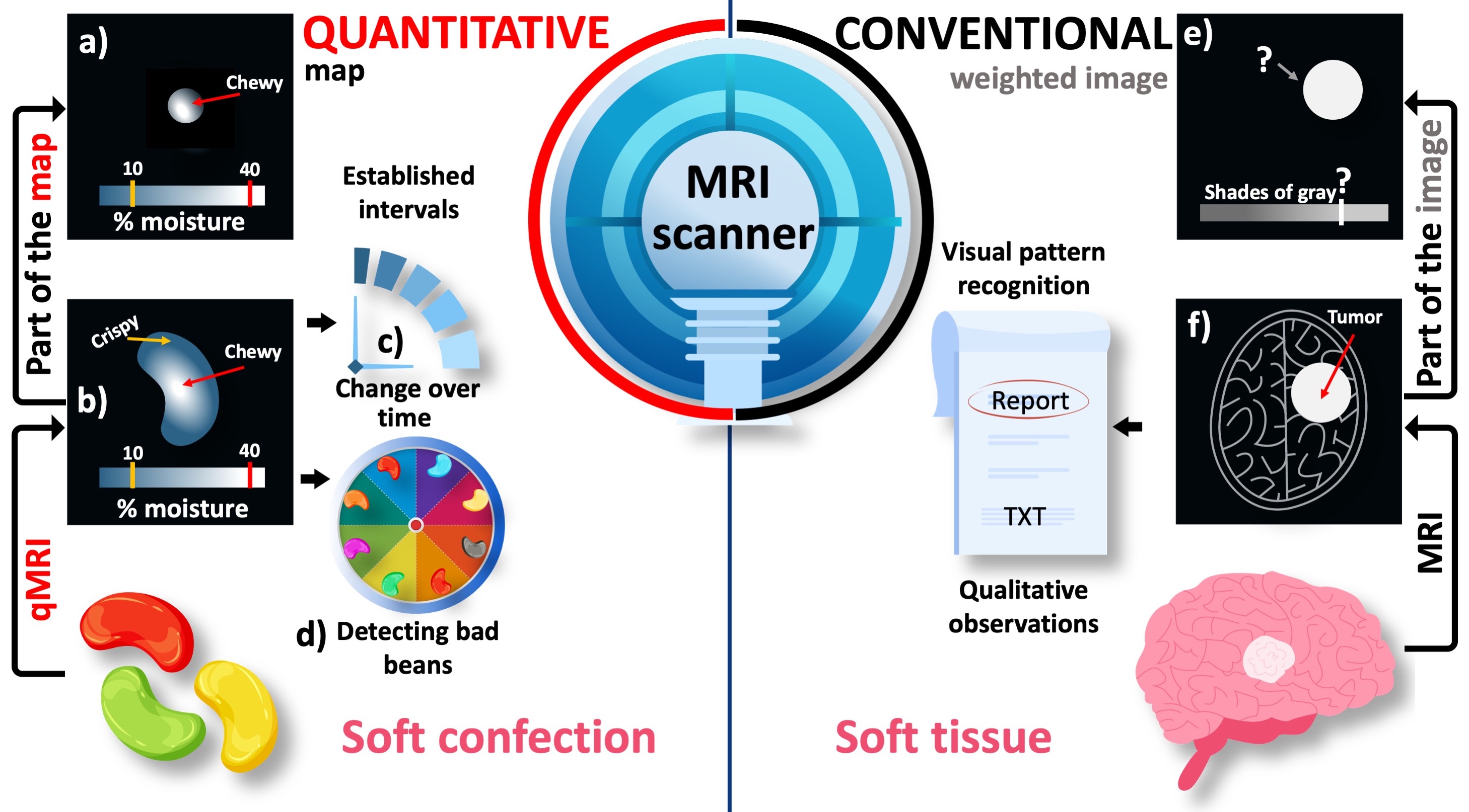
Figure 1:An illustrative comparison between the conventional and quantitative MRI (qMRI). The pixel brightness of conventional MR images is defined in an arbitrary grayscale (e,f). As a result, only a qualitative pattern recognition is possible when the suspected region (i.e., the tumor) is assessed against the background of the target anayomy (i.e., the brain). On the other hand, quantitative maps spatially resolve a meaningful metric (a,b) to detect changes over time (c) and between different samples (d). On a standardized measurement scale of percent moisture, the texture characteristics of a jellybean (e.g., crispy or chewy) can be objectively determined even from a randomly selected part of the image.
Using the same MRI scanner, it is possible to assign meaningful numbers to the images and this approach turns out to be the most common MRI method in food engineering Mariette et al., 2012Ziegler et al., 2003. Figure 1 illustrates the added value of quantitative MRI (qMRI) when applied to a sample familiar to everyone: a jellybean. The moisturization map indicates that the jellybean has formed a crispy shell while remaining chewy at the center, which is the desired texture Fig. 1b. Given that the level of chewiness is determined by a threshold on a standardized measurement scale, a randomly selected part of the image can be still characterized by comparing selected pixel values against the established threshold Figure 1. This feature of qMRI offers an objective insight into how the texture of this soft confection changes over time, which would help determine its best before date (Figure 1, prognosis).
The ability to reveal what underpins the appearance of visually similar samples is yet another powerful feature of qMRI. In a Bean-Boozled challenge, which is a Russian roulette of jellybean flavors, tasty flavors are mixed with nauseous look-alikes Gambon, 2015. For example, a green jellybean may taste like lime (tasty) or lawn clippings (nauseous) in the Bean-Boozled game Figure 2. Therefore, no matter how experienced the player is, the chances of picking up a lime-flavored bean is as good as tossing a coin. Conventional MR images of a handful of green jellybeans do not offer a distinguishing feature, but only reveal their structure. As a result, the chances of making an unfortunate choice remain the same Figure 2.
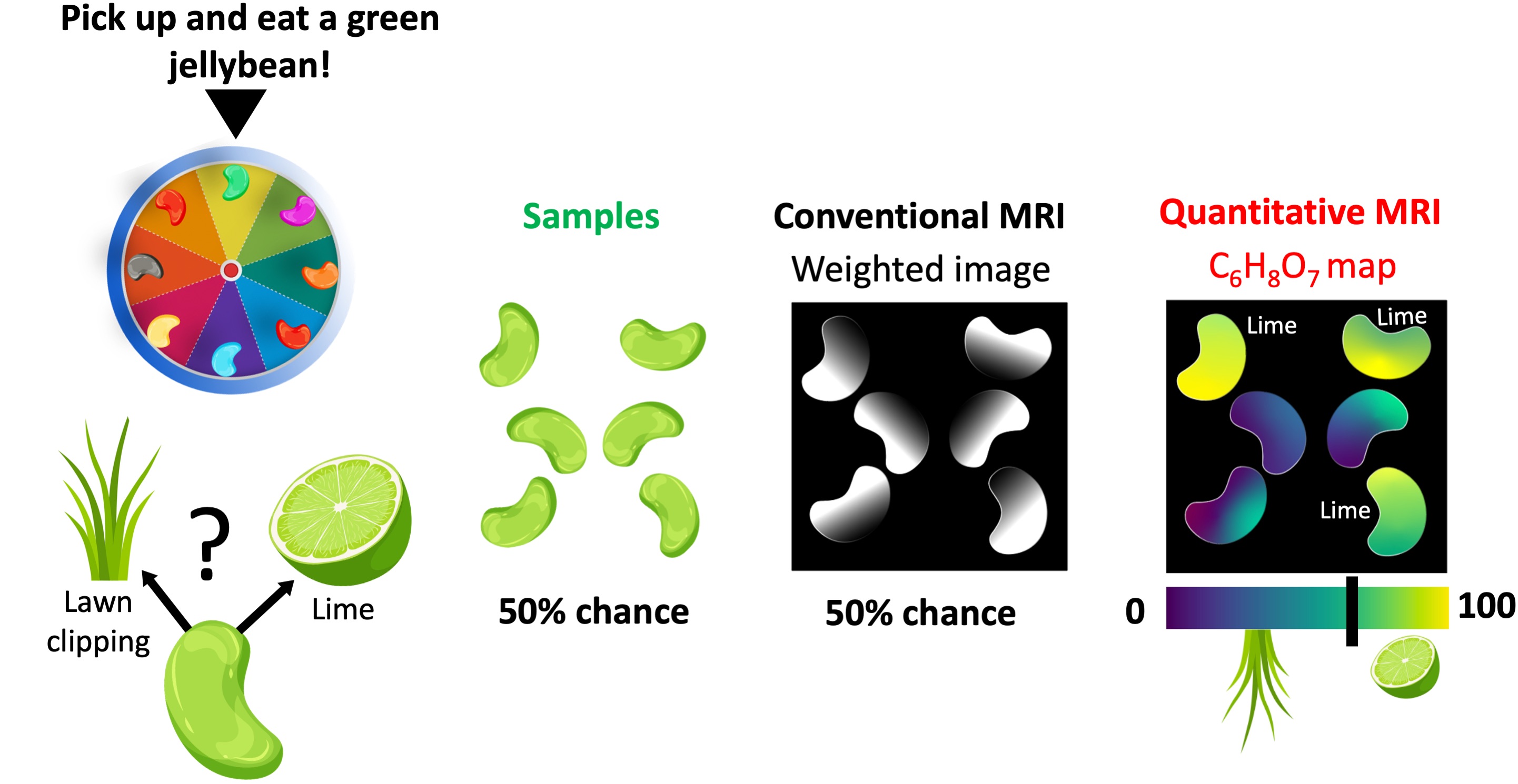
Figure 2:The comparison of conventional and quantitative MRI in a Bean-Boozled game, where the task is picking up and eating a green jellybean. Out of 6 green beans, half of them taste like lime (tasty) and the remaining are lawn clipping flavored (nauseous). Conventional MRI is not sensitive to either aroma, as a result the beans show similar contrasts. On the other hand, a quantitative mapping method sensitive to citric acid (C6H8O7) can help reveal lime-flavored beans.
On the other hand, spatially resolving a quantitative property that is sensitive to either flavor would step up our game in making the right decision. For example, a qMRI method capable of mapping the distribution of citric acid (C6H8O7) – the chemical compound that gives citrus fruits a sour taste – would help distinguish lime-flavored green beans. Even though the grass-flavored beans may contain a slight amount of C6H8O7 (used as lawn fertilizer), establishing a threshold can help make an informed decision (Figure 2), giving the players a competitive edge in the bean-boozled game (diagnosis).
Note that the pixel brightness of the conventional (weighted) image has contributions from the C6H8O7 concentration. However, it is also affected by several other factors, such as water density and glucose content. Therefore, understanding the relationship between the pixel brightness and the flavour depends on the experience and subjective interpretation of the observer.
NMR is a spectroscopy method that gives information about the chemical makeup of the analyzed substance. In analogy with the jellybean example, an NMR measurement is similar to quantifying the amount of C6H8O7 from the fragments of a green jellybean (Figure 2). If we used NMR for the bean-boozled challenge, we would be looking at a list of values to pick up a lime-flavoured bean instead of looking at a map.
1.2A spicy history of NMR and MRI
The evolution of NMR into MRI is a turbulent story Dreizen, 2004 that starts with the development of the first MRI scanner (1980) and leads to a Nobel Prize (2003). In 1971, Damadian published a study on the use of NMR-based T1 and T2 values for detecting malignant tumors Damadian, 1971. Based on this work, he issued a patent application titled “an apparatus and method for detecting cancer in tissue” in 1972, which was accepted in 1974 Damadian, 1974.
However, an actual image was out of the picture until Lauterbur was finally able to publish his work in 1973, showing a crude weighted-image of two liquid filled tubes Lauterbur, 1989. Lauterbur’s publication was delayed because the initial submission was desk-rejected by the editors of Nature, and his university did not find his work valuable enough to submit a patent Dawson, 2013. Around the same time but an ocean apart, Mansfield was applying NMR to image crystals by borrowing a concept dubbed k-space from 2D crystal structures Turner, 2017. This approach led Mansfield to develop a fast image generation method, bringing MRI closer to practical reality Mansfield & Maudsley, 1977.
With undeniable insight from the studies of Lauterbur and Mansfield, Damadian’s team built the first human MRI scanner in 1978 and made it commercially available in two years. Around the same time, GE started manufacturing scanners without paying royalty to Damadian as consideration for the patent. In the decade that follows, GE sold nearly 600 scanners, for which Damadian’s company Fonar filed a patent infringement lawsuit in the late 1990s and awarded $128,705,766 as a compensation for pecuniary damages (Cir., 1996).
1.3A bitter U.S. Supreme Court verdict
Returning to the jellybean analogy, Damadian’s patent was mainly describing a device to scan whole jellybeans for a complete C6H8O7 measurement. The key invention of the patent was to collect multiple measurements at different locations of the jellybean without fragmenting them. Later on, Lauterbur and Mansfield developed the methodology to create weighted images of the jellybeans. This was followed by Damadian marketing the first device that can generate weighted images of whole jellybeans (Figure 2) and the U.S. Supreme Court reached the verdict that GE infringed Damadian’s patent. The original judgement on the verdict reads:
On May 27, 1997 the Honorable Wm. H. Rehnquist, Chief Justice, the United States Supreme Court, enforced the Order of the Federal Circuit Court of Appeals and ordered GE to pay Fonar. GE paid Fonar $128,705,766 for patent infringement. GE was further restrained from any use of Fonar technology.” “The Court found that GE had infringed U.S. Patent 3,789,832, MRI’s first patent, which was filed with the U.S. Patent Office in 1972 by Dr. Damadian. The Court concluded that MRI machines rely on the tissue NMR relaxations that were claimed in the patent as a method for detecting cancer, and that MRI machines use these tissue relaxations to control pixel brightness and supply the image contrasts that detect cancer in patients.
To paraphrase the reasoning behind this decision using the jellybean analogy:
GE manufactured and sold 600 scanners capable of generating weighted images of the jellybeans,
the weighted images are influenced by the C6H8O7 concentration,
lime-flavored jellybeans have higher concentrations of C6H8O7,
thus, GE scanners are designed to identify lime-flavored jellybeans, which infringes on Damadian’s patent.
Although the U.S. Supreme Court decision implied that Damadian owns the intellectual property rights for MRI scanners at that time, the 2003 Nobel Prize in Medicine was shared between Lauterbur and Mansfied only. Damadian spent nearly $300,000 for full page ads in popular print media outlets to claim his rights to the 2003 prize, yet the situation has remained unchanged up to this date. The notes on why Damadian was not included in the prize will be available in 2053 Harris, 2003.
The court’s interpretation of the difference between the Fonar’s patent and GE MRI scanners perfectly captures the essence of qMRI, which is to enable objective and consistent comparisons by tagging each pixel with a precisely defined score that ranks a physical characteristic. Although the physical property estimated by qMRI contributes to the pixel brightness of conventional images, the conventional images are presented in an arbitrary grayscale. This is the reason why individual pixels of a weighted image have numbers, but no (physical) value.
To conclude, there is a critical difference between detecting abnormalities based on pixel brightness (conventional MRI) and tissue characterization using quantitative metrics (qMRI), and the court’s interpretation of this difference cost GE $129 million. With this central distinction in mind, the following sections will introduce how we can use the same MRI scanner for both qualitative and quantitative imaging.
2Origins of MRI - A Visual History
A pictorial and historic journey into how MRI works
The human body can be seen as a complex compartmentalization of water, fat, protein and minerals at every level of its organization from atoms to organs (Siri, 1956). At the atomic scale, nearly 63% of the atoms in the human body are hydrogen atoms (Osmera and Vanicek, 1940), which consists of only one proton and one electron. It is this simplicity that makes hydrogen the most studied atomic structure in quantum mechanics, which eventually lead to the development of MRI.
Once the mass and charge of the hydrogen particles were known, nobody suspected that there was another hydrogen property to be discovered. The study of hydrogen was revolutionized when two scientists in their mid 20s, Uhlenbeck and Goudsmit, wrote together the first article about the nuclear spin in 1925 (Uhlenbeck and Goudsmit, 1925). They were afraid to submit their work, because the celebrity physicist Lorentz deemed their idea “unphysical”. At that time, Uhlenbeck and Goudsmit were working under the supervision of Zeeman and Ehrenfest, yet Zeeman and Ehrenfest omitted their names from the article, deciding to use the youth of their protegees as a shield against any backlash (Halpern, 2017). What was feared to be a foolish mistake was then accepted as a built-in feature of any fundamental particle in the universe, just like the mass and charge. This quantum property – spin – is the key to understanding how MRI works.
2.1Getting on the same wavelength with a single hydrogen in the quantum realm
28 years before his student would give an underlying explanation, Zeeman showed that the energy levels in an atom change under the influence of a magnetic field, an effect known as Zeeman’s splitting (Zeeman, 1897). This is particularly important for hydrogen, because unlike a magnetic field, an electric field does not lead to an energy difference between its spin configurations (i.e., does not split) (Feynman et al., 2015). Hydrogen is assumed to have four (ground) spin states, created by the combinations of two up and two down spins from its proton and electron. Each combination constitutes a different energy level. The difference between these energy levels is so small that their separation is defined by the term “hyperfine splitting”. What encourages the hydrogen to exhibit more than one energy level is the presence of a uniform magnetic field (B0). This effect opens a communication line to interact with hydrogen, yet it takes some special effort to start a conversation.
2.1.1Picking up a hydrogen atom in the quantum realm: The perfect match
The hydrogen atom comes online only when standing up under the influence of a magnetic field (Figure 3a,b). The chances of getting a response from the hydrogen firstly depends on whether our message kindles just the right amount of excitement for it to switch between those hyper-finely separated energy levels (Figure 3). Although it almost seems like the hydrogen is sidestepping a conversation, all it takes is finding the right wavelength to meet this first requirement. Six years after the introduction of the spin concept, Rabi and Breit finally discovered that to resonate with hydrogen’s energy levels, we need to send our messages in the radiofrequency (RF) range of the electromagnetic spectrum (Breit and Rabi, 1931).
However, not all hydrogen atoms behave the same. We need to be familiar with the peculiarities of the hydrogen we are in touch with. There are two key attributes: where is the hydrogen from, and in which energy state it is when our resonating message is delivered (Figure 3c). The last nuance to get on the same wavelength is finding the right angle to approach it. If we meet all the requirements, we will see the hydrogen getting excited and responding to us within a certain RF bandwidth.
For the imaging of the human body using MRI, we will be mostly communicating with the hydrogen from the water (Figure 4). In general, water hydrogens are more easy-going because their electron spin states are balanced, so we are only concerned with the energy levels emerging from their nuclei. This is why we call this pick-up line the nuclear magnetic resonance (NMR).
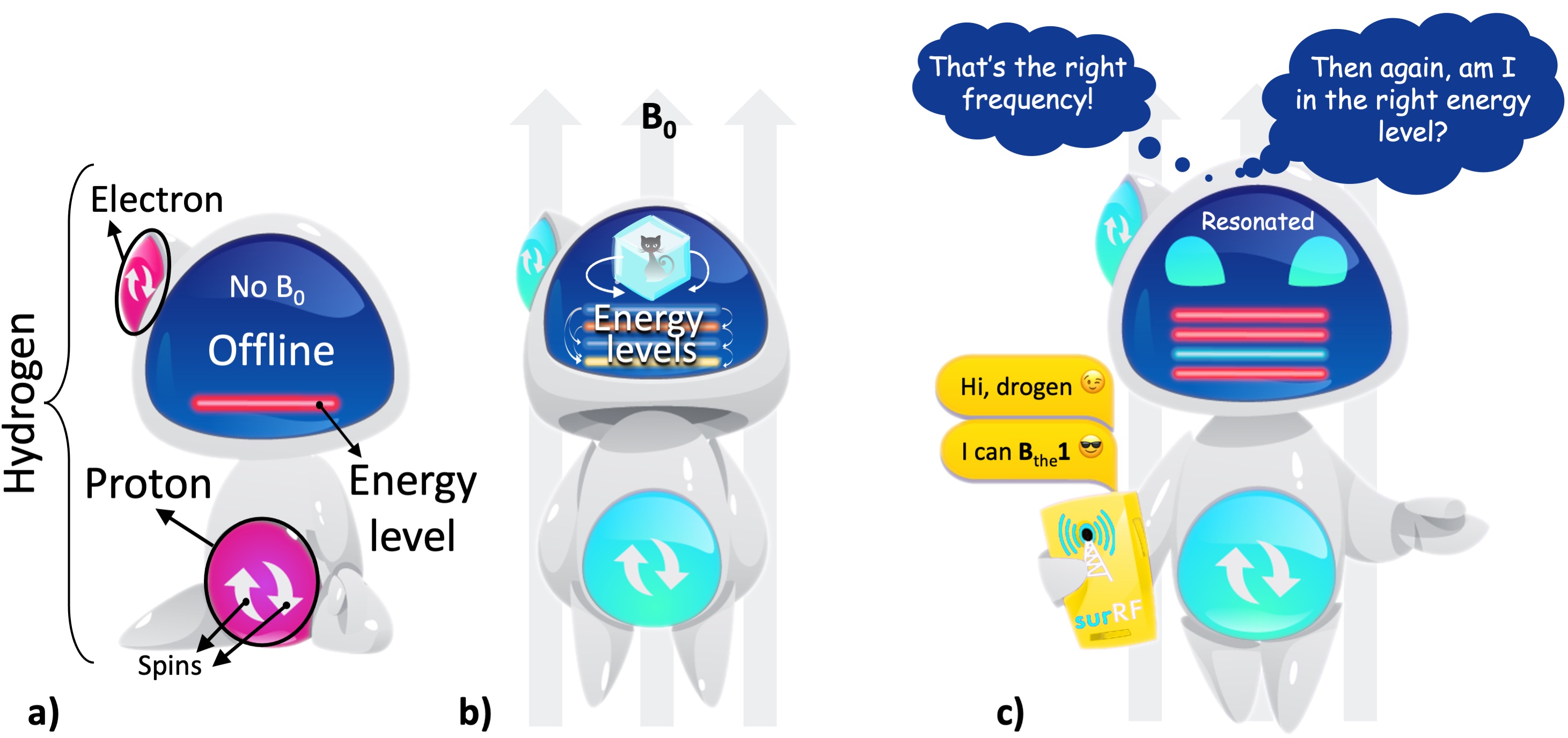
Figure 3:a) A hydrogen atom has one proton and one electron, with each particle is assumed to have two possible spin states for simplicity (up or down). In the absence of a magnetic field, the atom is at a random orientation (offline) and shows a single energy level (the red line). b) Under a uniform magnetic field (B0), the atom is aligned with the field (online) and shows multiple energy levels (the colored lines). These energy levels are in quantum superposition: all the levels simultaneously exist and we can only determine one state upon observation. This behaviour of the energy levels is represented by the Schrödinger’s cat2. c) Once it is online, the hydrogen atom can be contacted through a communication line that operates within the radiofrequency (RF) range.
Figure 4 shows that the hydrogen from water has two energy levels under a uniform magnetic field: low energy and high energy. If the resonating message flips the hydrogen’s energy state from higher (red) to lower (cyan) state, the result is a “radio silence” (Figure 4a), i.e. the hydrogen gives up a small amount of excess energy instead of a response. But if the resonating message elevates the hydrogen’s mood from lower (red) to the higher (cyan) state, the hydrogen gets excited (Figure 4b). After the message is delivered, we will finally get a response as the excitement quickly fades away. This final process is termed “relaxation”, which is of essence to the MRI contrast, because the message carries information about where that hydrogen is from.
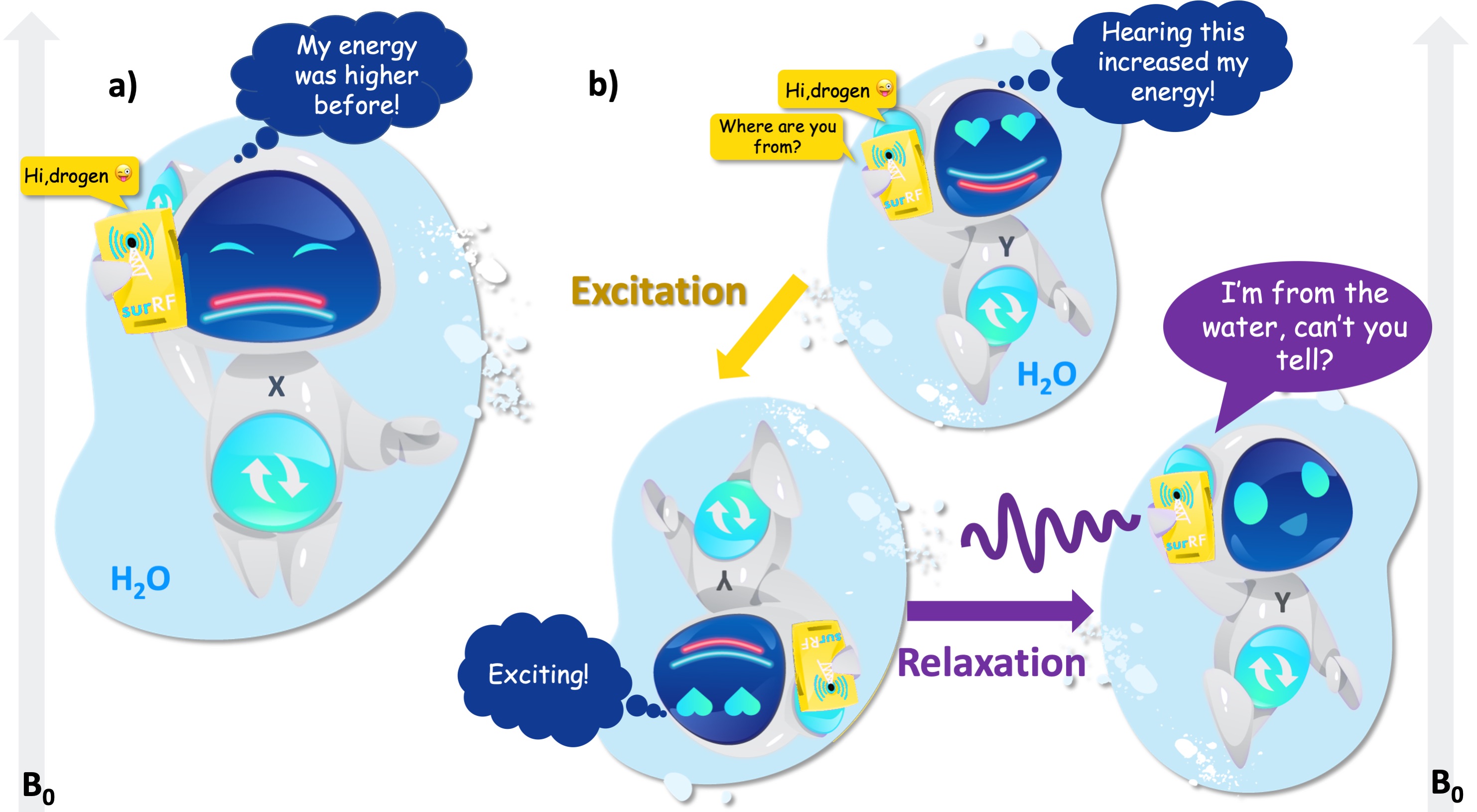
Figure 4:a) After receiving the call, the hydrogen atom from water switches from the higher (red) to the lower (cyan) energy level and refuses to answer. b) When the RF input switches its energy from the lower (red) to the higher level (cyan), the atom gets excited. While returning to its initial state, the atom responds.
The tone in the response shifts slightly if the hydrogen is from non-water molecules, e.g., fat or protein. This slight difference is caused by the amount of negative energy a hydrogen is surrounded by, which interferes with the contribution of hydrogen’s electron to its energy state, namely shielding. The more negative energy around the hydrogen, the shorter the response. It appears that the positive effects of being near water on the energy levels tran- scends scales, from humans themselves (Cracknell et al., 2016) to the hydrogen atoms that make up them (Lawrence and McDonald, 1966).
So far we looked at the quantum-level interactions between the hydrogen atom and RF energy, and tied it with the NMR phenomenon. However, in reality, we don’t have access to observed NMR effects at such a fine-grained level; because no appropriate instrumentation exists, and quantum-jitters make such instrumentation nearly impossible (Erkintalo, 2021). For example, we cannot detect the uncertainty of a single hydrogen atom’s energy levels. The best we can do is to visualize the concept using metaphorical illustrations, such as using Schrödinger’s cat to imply the quantum state of the hydrogen’s energy levels in Figure 3b. Until we observe the consequences (whether the hydrogen will respond to our resonant message or not), all the energy levels are assumed to be in quantum superposition, even for only two energy states of proton spins as shown in Figure 4. To achieve observational accuracy, we need to move from the uncertainties of the energy levels to a probability of getting a response to our resonant message, which is what we will look at in the following section.
2.1.2Finding the perfect quantum match is not practical, but there are plenty of fish in the sea
We can harness the benefits of NMR without having a complete theoretical understanding of the underlying quantum interactions (see proton spin crisis (Siegel, 2017)), because these effects simply smooth over at the macroscale. At this point we will leave the online dating analogy behind, because even at the smallest macroscopic scale, “there are plenty of fish in the sea” (Figure 4a). At the level where an NMR measurement is technically feasible, we will be concerned with a large pool of hydrogen atoms. Here, the individual behaviour of particles becomes useless for characterizing the system in aggregate. This concept of integrating over microscopic details to achieve a compact and useful system description is coarse-graining (Figure 5).
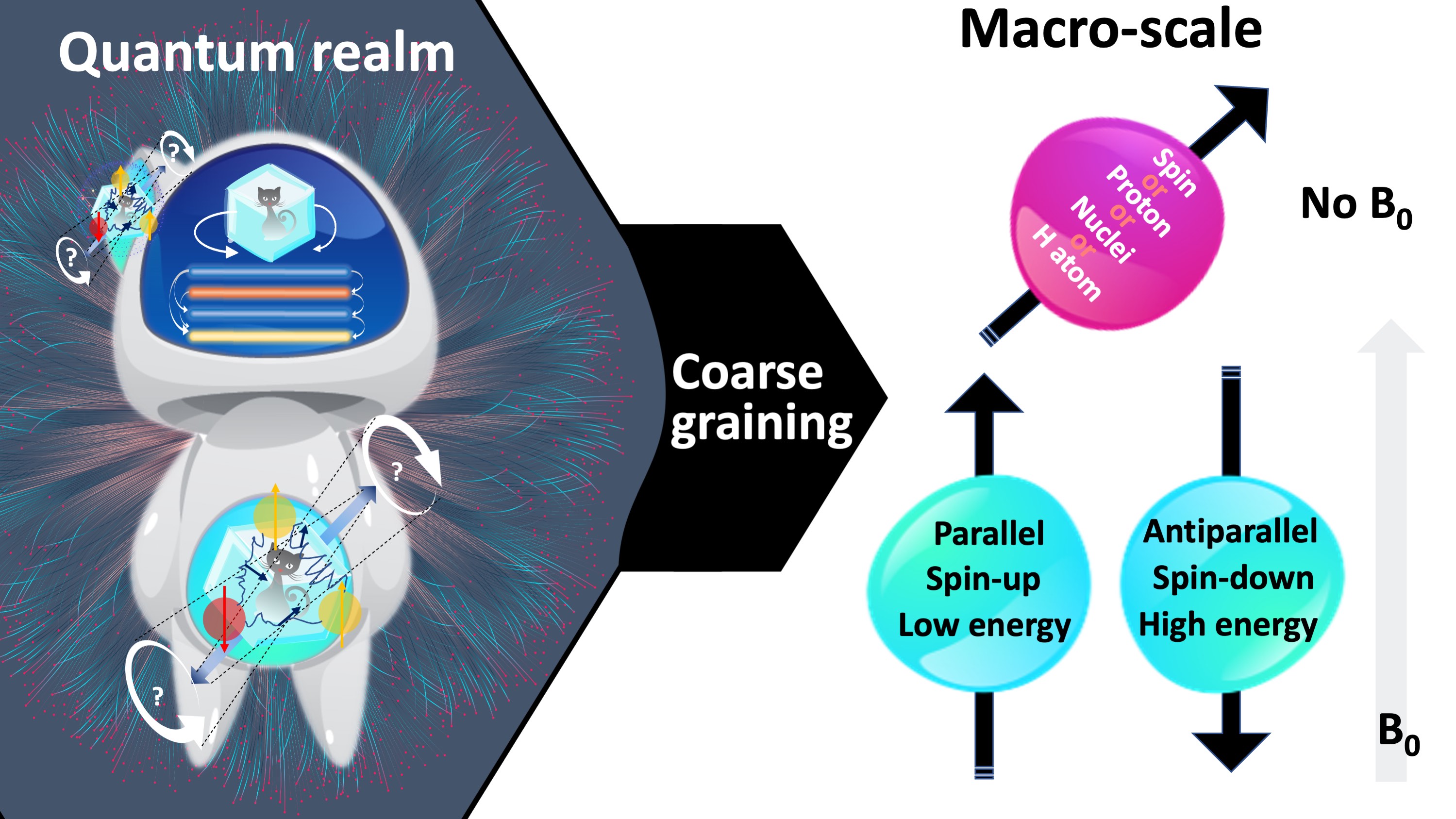
Figure 5:At the macro-scale, the quantum mechanical behaviour of individual hydrogen atoms is averaged over, i.e., coarse-grained. Figure 2 illustrates a fine-grained description of the behaviour of a single hydrogen atom in absence and presence of a magnetic field. After coarse graining, the representation simplifies to an arrow passing through the center of the proton, which is aligned parallel (i.e., spin-up, low energy) or antiparallel (i.e., spin-down, high energy) with the magnetic field (blue), or at random if the field is absent (pink). Follow- ing coarse-graining, the terms spin, proton, nuclei or hydrogen can be used interchangeably.
Figure 5 shows how the representation of a hydrogen atom is changed after coarse-graining microscopic details of spin interactions. From this point onward in this document, hydrogen will be illustrated as shown in Figure 5, and used interchangeably with the terms spin, proton and nuclei. To refer to the energy level associated with a single hydrogen atom, we will describe the magnetic moment (Figure 6a): If the proton was merely a rigid body, its rotation about an imaginary axis that passes through its center would create a small angular momentum aligned with that axis. Given that the proton is a charged particle, it also creates a microscopic magnetic moment (μ) as a result of this rotation, which is a vector in the same direction (Figure 6a). The ratio between the angular momentum and the magnetic moment yields the gyromagnetic ratio (γ), which is 42.59 MHz for the hydrogen at 1 Tesla (T) magnetic field. This frequency at which the spins rotate is commensurate with the magnetic field strength. The product of the gyromagnetic ratio and the field strength (γB0) yields the Larmor frequency, at which the RF energy must be delivered to achieve nuclear resonance.
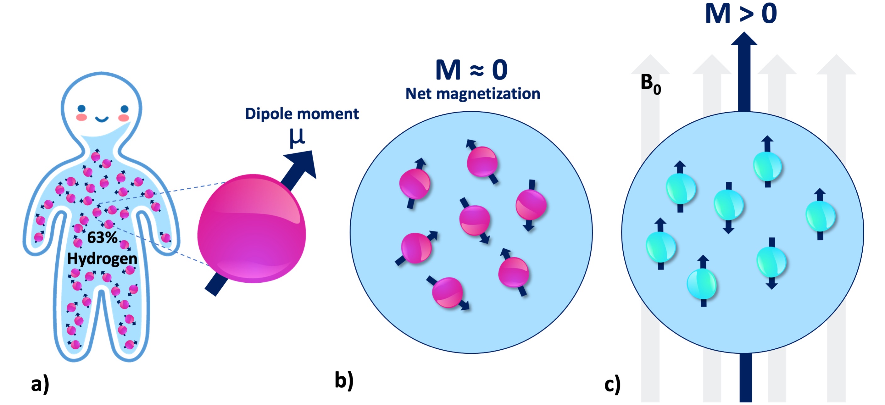
Figure 6:a) There are millions of protons (i.e., spin or nuclei) even at the smallest macro- scopic unit volume relevant to the MR imaging of the human body. Each individual proton exhibits an infinitesimally small magnetic moment (μ). b) Without B0, the protons in a spin pool exhibit random alignment. c) In presence of B0, the spins are aligned with the magnetic field (parallel or antiparallel), giving rise to a net magnetization (M).
At the macroscale, we will be concerned with millions of protons at once (Figure 6a), even for a unit volume of 1mm3. Absent an external magnetic field, magnetic moment vectors are oriented at random (Figure 6b). When a magnetic field is applied, they are aligned either parallel (spin-up, low energy) or antiparallel (spin-down, high energy) with the applied field (Figure 6c). Given the vast abundance of these spins, the relevant question becomes: which spin configuration is dominant? According to the second law of thermodynamics, if the spin system is at thermal equilibrium, i.e., no energy enters or leaves the system, the entropy of that spin system increases (Carnot et al., 1899). This omnipresent tendency toward disorder favors low energy (Ferris, 2019). Therefore, the spin system tends to have slightly more low-energy hydrogen atoms (spin-up, parallel). Although the difference is as small as 40 per million protons (Webb, 2016), a net magnetic magnetization (Figure 6c) can be observed by a real-world NMR experiment.
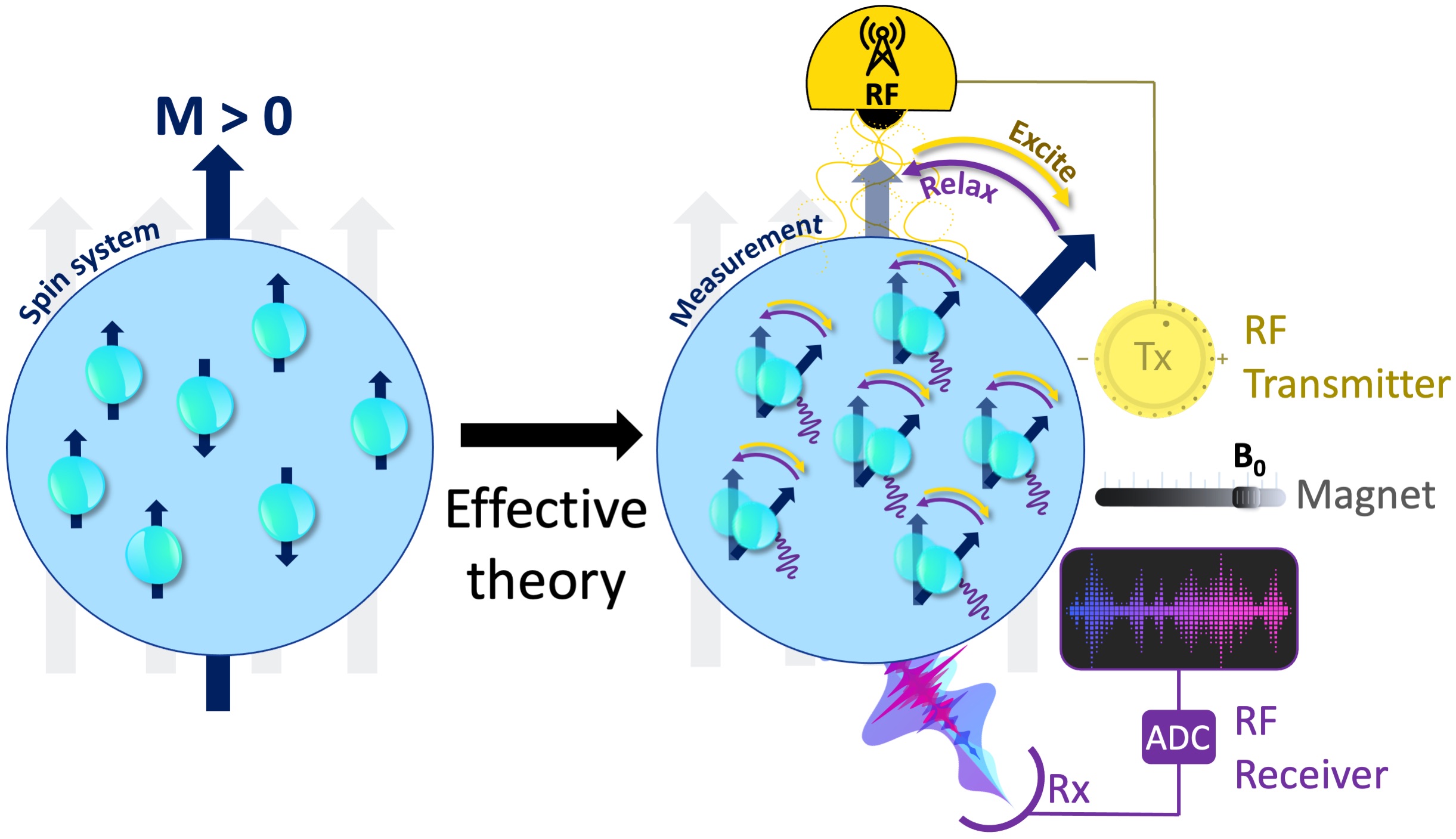
Figure 7:The measurement instrumentation is concerned with the relevant degrees of free- dom and an effective theory that explains how these coarse-grained variables respond to the perturbations of the measurement system. Some fundamental components of an MRI mea- surement include a uniform magnetic field generator (i.e., a magnet), an RF transmitter (Tx, yellow), an RF receiver (Rx, purple) and an analog-to-digital converter (ADC).
To perform a real-world measurement, an effective theory is needed to describe how the coarse-grained features of the targeted system (Figure 6) changes upon interaction with the measurement instrumentation (Figure 7). The effective theory of relaxation for the bulk magnetization M was described by Felix Bloch in 1957, laying one of the cornerstones to bring MRI to reality (Bloch, 1957). A basic instrumentation to study the relaxation of a spin system is depicted in Figure 6c, including a uniform magnetic field (B0) generator, an RF transmission system tuned to the Larmor frequency and an RF receiver coil followed by an analog-to-digital converter (ADC). The following section describes how Bloch equations explain the macroscopic behaviour of the net magnetization and how MRI scanners make use of this effective theory to create images.
3From spin dynamics to images
Measuring and encoding the MRI signal
3.1Mathematical Description of Spin System Evolution
Following an excitation of the spin system by an RF energy at the Larmor frequency (γB0), the macroscopic Bloch equation describes how net magnetization evolves over time in a fixed cartesian reference (xi, yj, zk), under B0 is given by:
where M0 is the initial magnetization of the spin system and T1 and T2 are the time constants for the longitudinal and relaxational components of relaxation. The first term of the Eq. 1 is precessional, and the last two terms are the relaxational components of the Bloch equation. Recall that in thermal equilibrium, the net magnetization is aligned with the applied magnetic field (Figure 6c), where the longitudinal component is the net magnetization (M = Mz = M0) and the transverse component equals zero (Mx = My = 0). In this case, the last two terms of the equation vanish, leaving the precessional component of the equation. When the phenomenological Eq. 1 is solved for the longitudinal (Mz) and the transverse (Mxy) components of the macroscopic magnetization, the explicit solutions are given by:
Note that Eq. 2 describes an exponential recovery for Mz to return the equilibrium after excitation. On the other hand, Eq. 3 states that the transverse magnetization follows an exponential decay, quickly converging to zero.
3.2Analogical explanation using a defibrillator
The relationship between the longitudinal and transverse components of magnetization in an NMR experiment can be understood through the analogy of how a defibrillator’s capacitor charges and discharges. As soon as the paramedic hits the shock ⚡️ button, the capacitor abruptly empties to deliver an immediate and strong jolt to the patient (Figure 8). At this moment, the paramedic’s focus is on how the energy dissipates across the patient’s body, which lies in the transverse plane (Mxy). The time it takes from the start of the shock until 37% of the energy remains (1/e = 0.37) corresponds to the T2 time constant of Mxy. This process is very brief, similar to the sound of a click.
After delivering the shock, the capacitor must recharge to the desired level to be ready for the next shock (Figure 8b). The time required for the capacitor to reach 63% of its total charge capacity (1-1/e) corresponds to T1 time constant of the Mz. This recharging process is slower and is often accompanied by a rising whine or whirring sound, indicating the gradual buildup of energy.
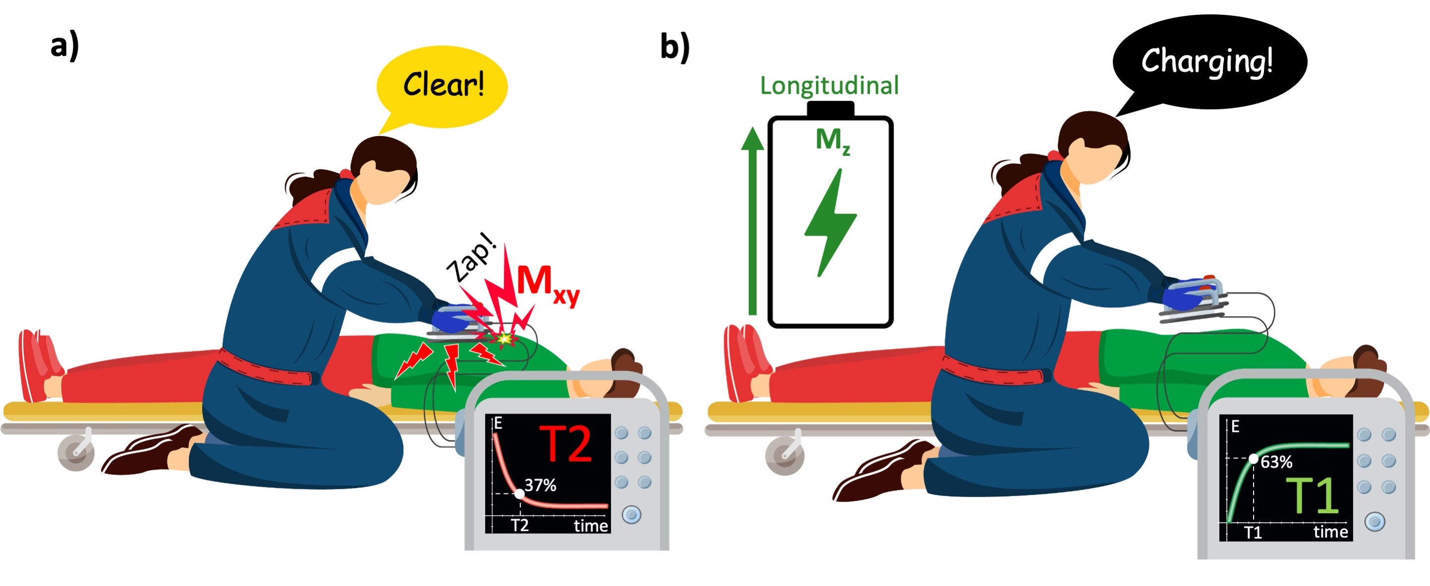
Figure 8:Time-dependent behavior of the transverse and longitudinal magnetization can be compared with how the capacitor of a defibrillator empties and recharges. a) When the paramedic activates the shock paddles, the capacitor quickly discharges its energy to the transverse plane (patient’s body). b) To deliver the shock again, the capacitor must be recharged, which happens quickly, yet relatively much slower than it discharges.
3.3Extending the defibrillator analogy to measurement instrumentation
The use of the defibrillator by a paramedic highlights the distinct nature of T1 and T2 relaxation times in the context of energy dissipation and recovery in a repetitive process. However, it lacks the measurement aspect of an NMR experiment.
To complete the analogy, we will design a calibration setup to measure the energy delivered to the patient’s torso. To measure this indirectly, a loop will be placed under the stretcher and the current induced in the loop as a result of the delivered shock to the patient’s body will be recorded (Figure 9). The signal observed at the end of each shock corresponds to the free induction decay (FID) in an NMR experiment.
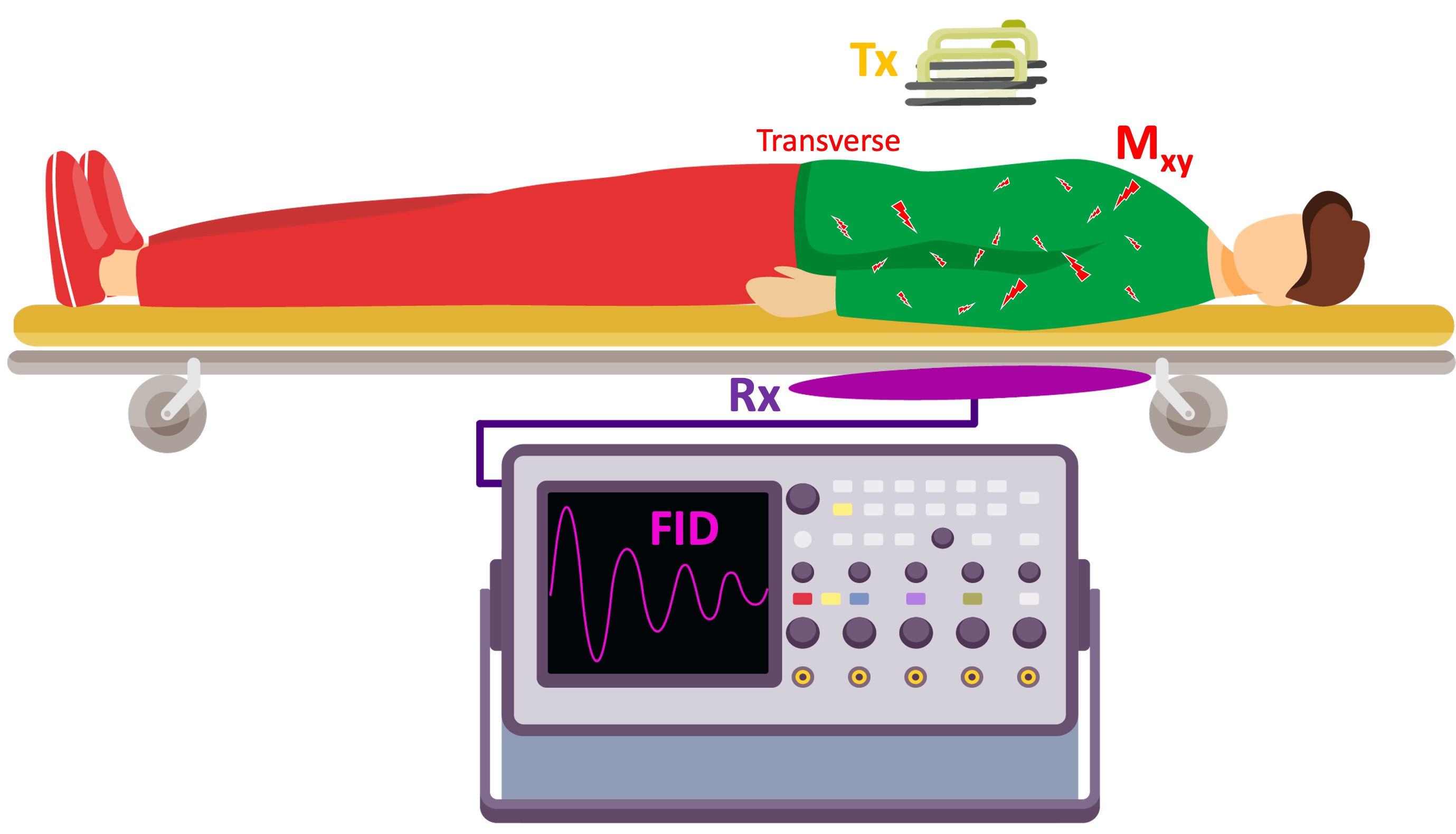
Figure 9:A hypothetical calibration setup: To have a measure of the energy delivered to the patient, a conductive loop is placed under the stretcher. After the shock is delivered, the current induced in the loop is captured by a oscilloscope.
If the biochemical composition of the excited volume varies spatially, the measured FID will be a summation of slightly varying frequency components. For example, a hydrogen atom from the water has a longer response than a hydrogen from the fat (T2fat<T2water). When the frequency components of the FID are observed by applying a Fourier transform, the respective peaks will be separated by a certain extent in the NMR spectrum, depending on the field strength (Figure 10).
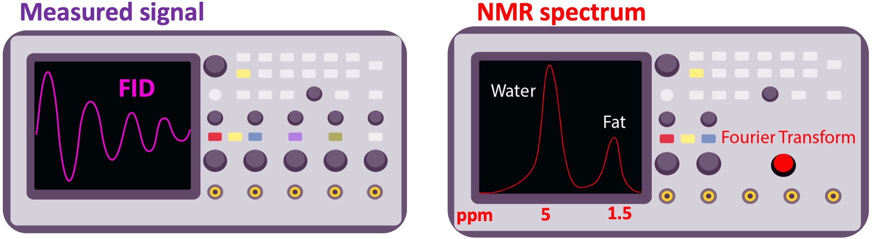
Figure 10:The free induction decay (FID) signal (left), and its frequency spectrum (right). As the electron of the hydrogen atom is more shielded in fat, its peak appears on the lower end (right, by convention) of the chemical shift spectrum. The chemical shift of water and fat is separated by 3.5 part-per-million (ppm), which corresponds to 146 Hz frequency difference at 1T ().
With the ability to precisely reveal molecular signatures, NMR is one of the most popular methods of chemical spectrum analysis, which is still in active use for a broad range of applications. A familiar example would be the benchtop NMR spectrometers at the airports that are used for tracing explosives and narcotics. However, spectral analyses take place in one dimension, in which the application of magnetic resonance was restricted for 25 years.
3.4From the peaks of frequencies to a bright spot in an image: Spatial localization
A magnetic field gradient refers to a gradual change in B0 in any desired direction. This is achieved by flowing high-amplitude electric currents through coils installed in three orthogonal directions. For example, Z gradients (head-foot direction) are a pair of circular Helmholtz coils (green rings in Figure 11) that can generate a gradually increasing or decreasing magnetic field by running currents in opposite directions. The higher the current, the steeper the magnetic field difference between the opposite ends of the scanner’s bore. The magnitude of this gradient field can be adjusted such that the spins precess at the Larmor frequency of B0 only at a certain region (selected volume). This way, only the spins from the selected volume will absorb the RF energy deposited at the resonance frequency. To achieve this “spatial localization”, the RF transmitter is turned on concurrently with the gradient coils, sustained briefly (typically in a micro- to milliseconds scale), then turned off. Operating hardware components in this fashion is termed playing (RF or gradient) pulses. Timing of such events is described by pulse sequence diagrams.
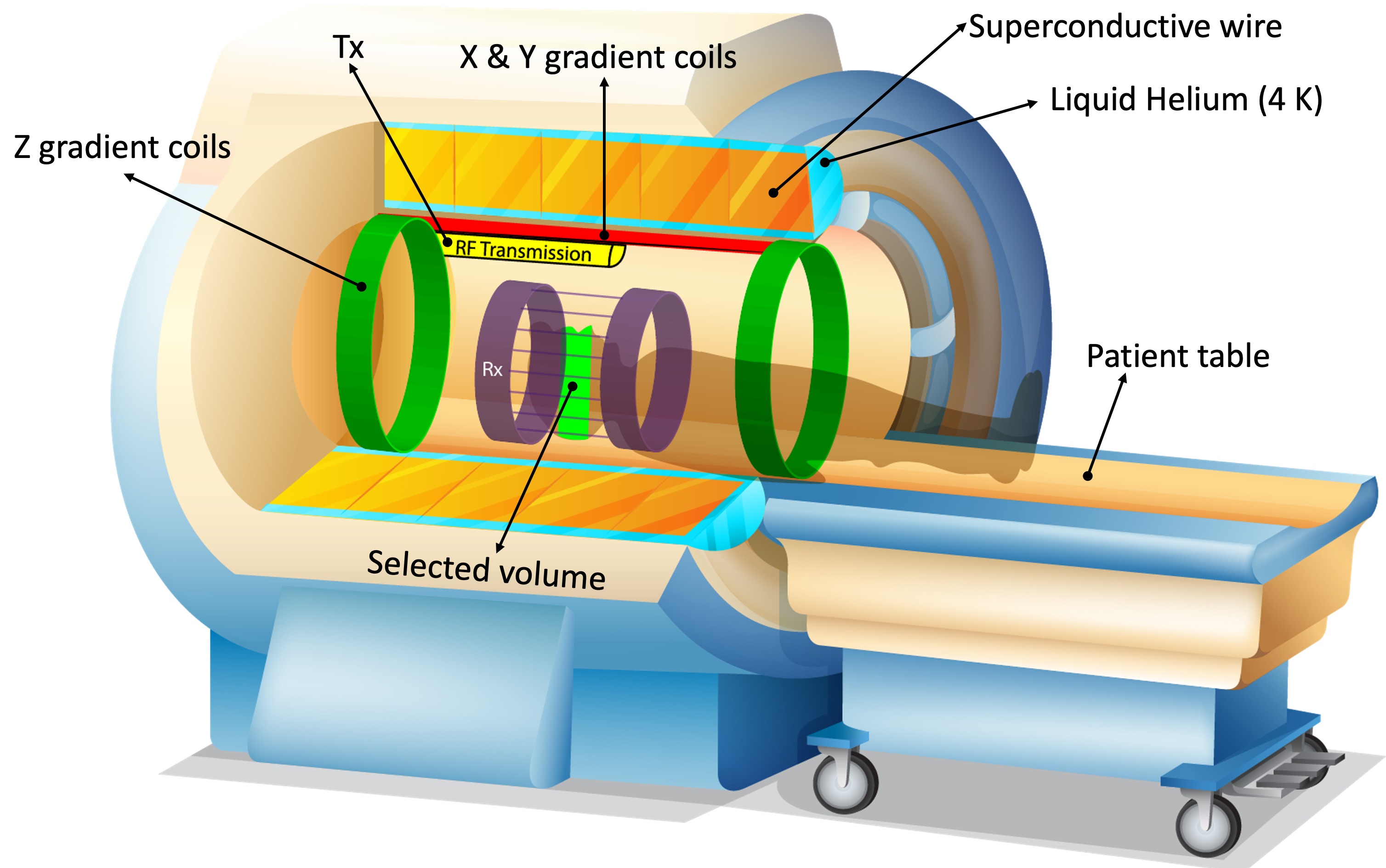
Figure 11:Hardware components of a modern MRI scanner using a superconductive magnet. Z-axis gradients (green rings) spatially vary the magnetic field, such that only the spins at a limited region (light green area in the patient’s head) precess at the Larmor frequency (γB0).
Figure 12 shows the sequence diagram describing the spatial localization illustrated in Figure 11.
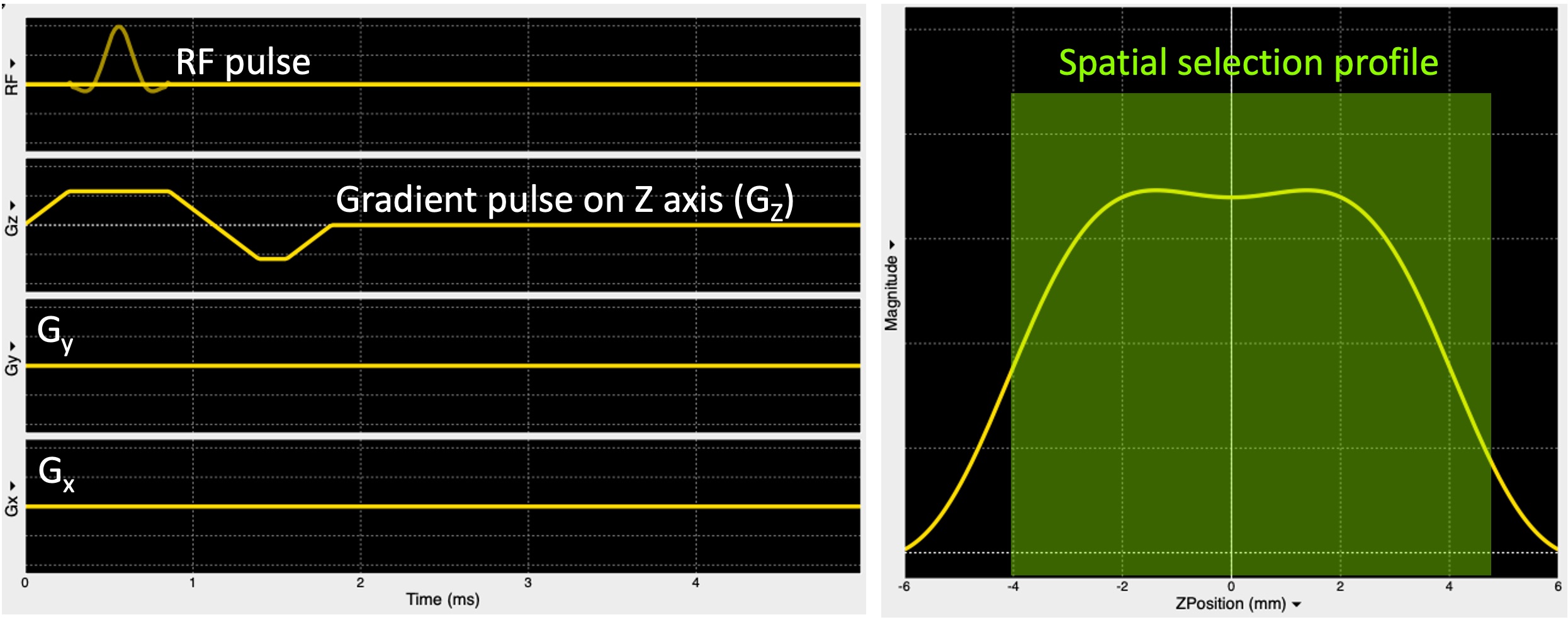
Figure 12:A pulse sequence diagram (left) showing an RF pulse to excite the spins only in a plane selected along the z-axis (Gz) and the respective slice profile (right).
However, the slice selection procedure does not encode the measured signal with positional information. If an ADC event (i.e. signal measurement) was followed soon after the RF pulse was turned off, the receiver coil (Rx, purple, Figure 11) would collect information from the whole excited region at once. To form an image, the received signal must be encoded in-plane, which is along the x (row) and y (column) axes (axial plane) for the selected region.
Figure 13b explains how spatial encoding in the row direction is performed by playing a gradient along the x-axis (Gx, teal) while the signal is being measured (ADC, purple). As a result of this, spin locations across a single row (the red box outlined in Figure 13c) are uniquely sorted out as a function of their frequency, namely the frequency encoding. The process of acquiring data using frequency encoding is termed a readout (purple box) and the acquired data is referred to as an observation (Figure 13d). During a readout, the receiver coil picks up a sinusoidal electromagnetic signal as an observation (purple sinusoid in Figure 13d), composed of the frequency components encoded per voxel (blue sine waves in Figure 13d). Therefore, the ADC must ensure that the observation is sampled at a high enough rate to resolve all 10 frequency components. In this example, the observation must be sampled at least at 20 locations to satisfy the Nyquist condition (purple squares in Figure 13d). The ADC hardware of modern MRI scanners is fast enough to achieve high sampling rates up to 500kHz (Graessner, 2013) and smart enough to perform an IQ sampling, separating the magnitude and phase components of each data point (Kirkhorn, 1999). This offers the convenience to place an observation to its location in a special data plane: the k-space (Figure 13e).
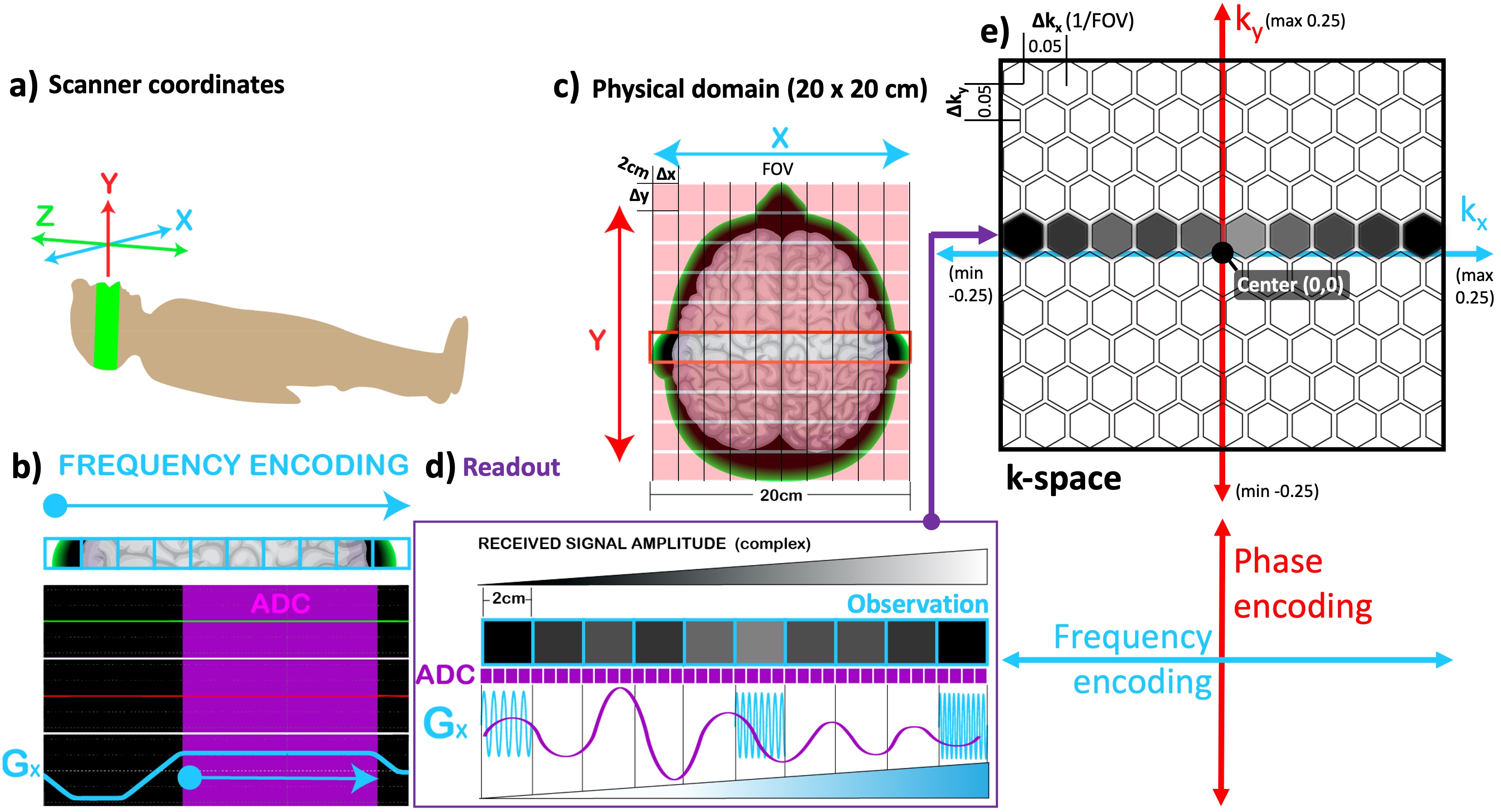
Figure 13:The correspondance between the scanner coordinates (a) and the selected imaging plane (c) is illustrated along with the pulse sequence diagram for frequency-encoding (b). The observation obtained by the readout (d) is shown in the k-space (e).
By convention, the location in the horizontal axis of the k-space is determined by the spatial frequency and the value of each cell is proportional with the magnitude of the respective signal component. The k-space is arranged such that the higher frequency components are located around the skirts, whereas the lower frequency components are closer to the center. In a sense, placing an observation in its k-space location corresponds to adding in the contribution of that acquired portion to the whole image, but in the frequency domain. Hence, there is not a pointwise correspondence between the k-space and the MR image it represents. Instead, every single cell in the k-space (each hexagon in Figure 13e) carries information about the whole image. The concept of k-space involves several layers of abstraction that are beyond the scope of this introduction; therefore, the reader is referred to (Mezrich, 1995) for an intuitive understanding of k-space. For the next step of our MR image generation example, we will be concerned with how to fill out multiple rows of the k-space (along the red axis).
Recall that an excitation RF pulse nudges all the spins toward rotating synchronously, so that Mxy across all the pixels share the same phase. Whenever a gradient is played, an opposite effect comes into play: phase of the spins along the gradient direction experiences a location-dependent shift. Each phase shift moves the location of the observation in k-space along the ky axis (Figure 14c), upwards or downwards depending on the polarity of the applied gradient. The amount of dephasing (i.e., the number of ∆ky steps) is proportional with the gradient area, and its effect can be rewinded to restore the transverse magnetization by playing a gradient of the same area with opposite polarity. Figure 14b shows a phase-encoding gradient (red) played with negative polarity before the readout in order to shift the observation to the next lower row in the kspace (Figure 14e). To rewind this dephasing effect, the readout is followed by another Gy gradient with positive polarity.
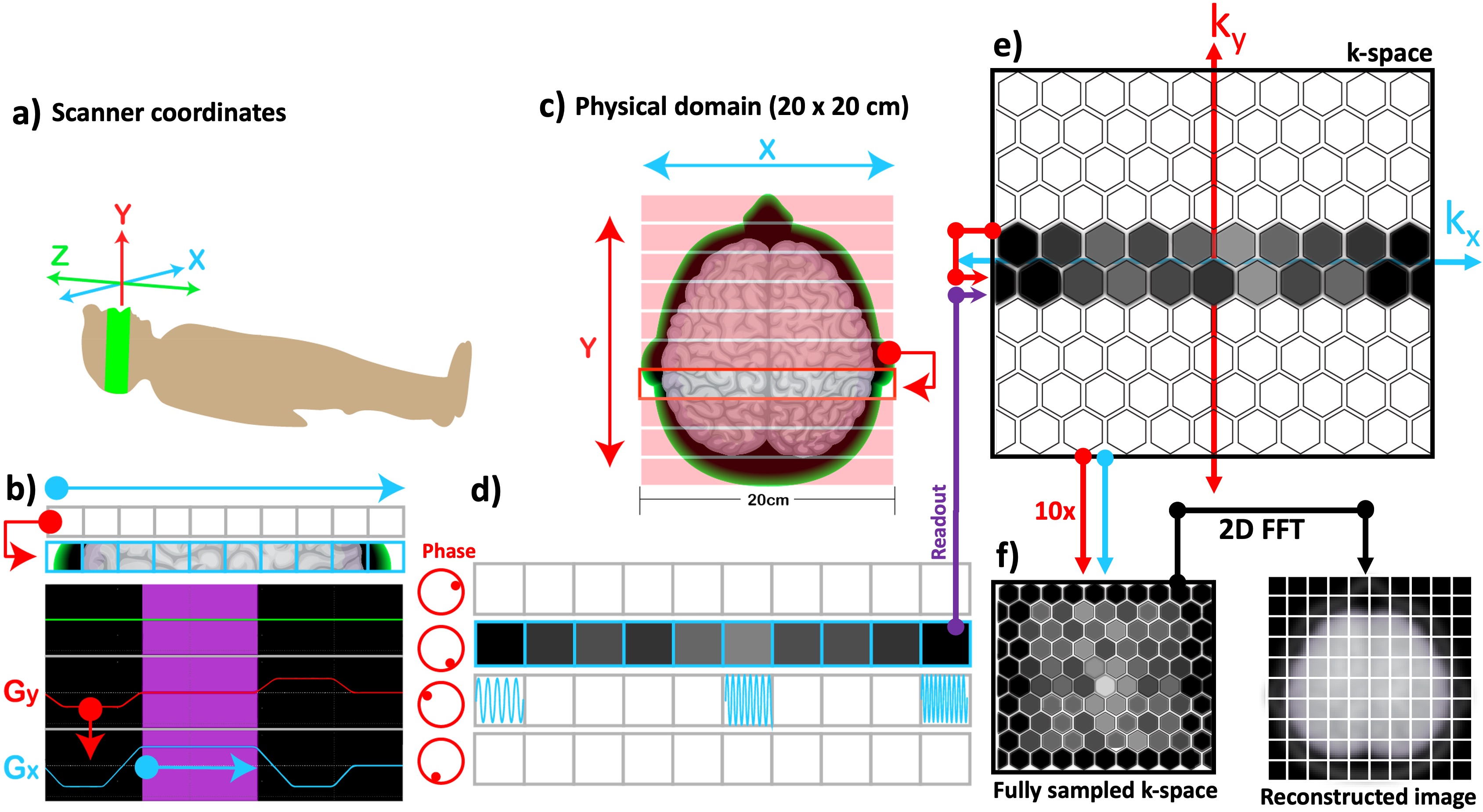
Figure 14:The correspondence between the scanner coordinates (a) and the selected imaging plane (c) is illustrated along with the pulse sequence diagram for phase encoding (b). Once the whole k-space is sampled by incrementing the phase-encoding gradient (red) (b) multiple times, a 2D inverse Fourier transform is applied to reconstruct the MR image (f).
By altering the gradient amplitude stepwise, the whole k-space can be sampled (Figure 14f). Therefore, the time that it takes to scan the plane shown in Figure 14c is a product of the number of rows and the duration of each repetition, namely the repetition time (TR). Finally, the MR image is reconstructed by applying a 2D inverse Fourier transform to the fully sampled k-space, where each sample corresponds to a grid location.
For the sake of simplicity, the examples in Figure 13 and Figure 14 assumed that the signal observations followed by an excitation pulse can be used to form an image. However in practice, an FID signal is short-lived; therefore, it cannot directly contribute to reconstructing an MR image. This brings us to two milestone discoveries in NMR by Erwin Hahn, which echoed into the beginning of MRI from a quarter-century behind and have become an indispensable part of its everyday use since then: spin- and gradient-echo. For further reading on the history of these methods, the reader is referred to an MRM Highlights interview with Erwin Hahn (Feinberg, 2018).
4Two MRI sequences and two qMRI measurements
Coming full circle back to two measurements with two pulse sequences
“The Court concluded that MRI machines rely on the tissue NMR relaxations that were claimed in the patent as a method for detecting cancer, and that MRI machines use these [T1 and T2 values] to control pixel brightness...” (GE vs Fonar 1996, U.S. Fed. Cir.)
Although going from values to brightness and back again is a 🐓&🥚 problem, GE could have stood a better chance by defending that the pixel brightness can be used to obtain T1 and T2 values, but T1 and T2 values cannot be directly utilized to obtain pixel brightness by MRI machines. Indeed, T1-weighted and T2-weighted contrasts are primarily determined based on the contribution of T1 and T2 (or neither). Nevertheless, to adjust those contributions, MRI machines use pulse sequences and parameters. This section will introduce two essential sequences, spin-echo and gradient-echo to show how contrasts are determined (conventional MRI) and the values are calculated (qMRI).
4.0.1Spin Echo and T2 mapping
In their seminal article titled “atomic memory”, Brewer and Hahn introduce the spin-echo (Hahn, 1949) by tapping into an intellectual conflict between the 2nd law of thermodynamics and the time reversal symmetry (Brewer and Hahn, 1984). The discussion is illustrated in Figure 15 to portray the paradoxical nature of the discussions on the physical phenomenon giving rise to a spin-echo. This is yet another effect exploited by the MRI, without necessarily having a complete understanding of the underlying “hidden order” effect emerging from the microscale interactions. For further reading on the conflict between the time symmetry and the entropy, the reader is referred to a recent blog post (Siegel, 2019).
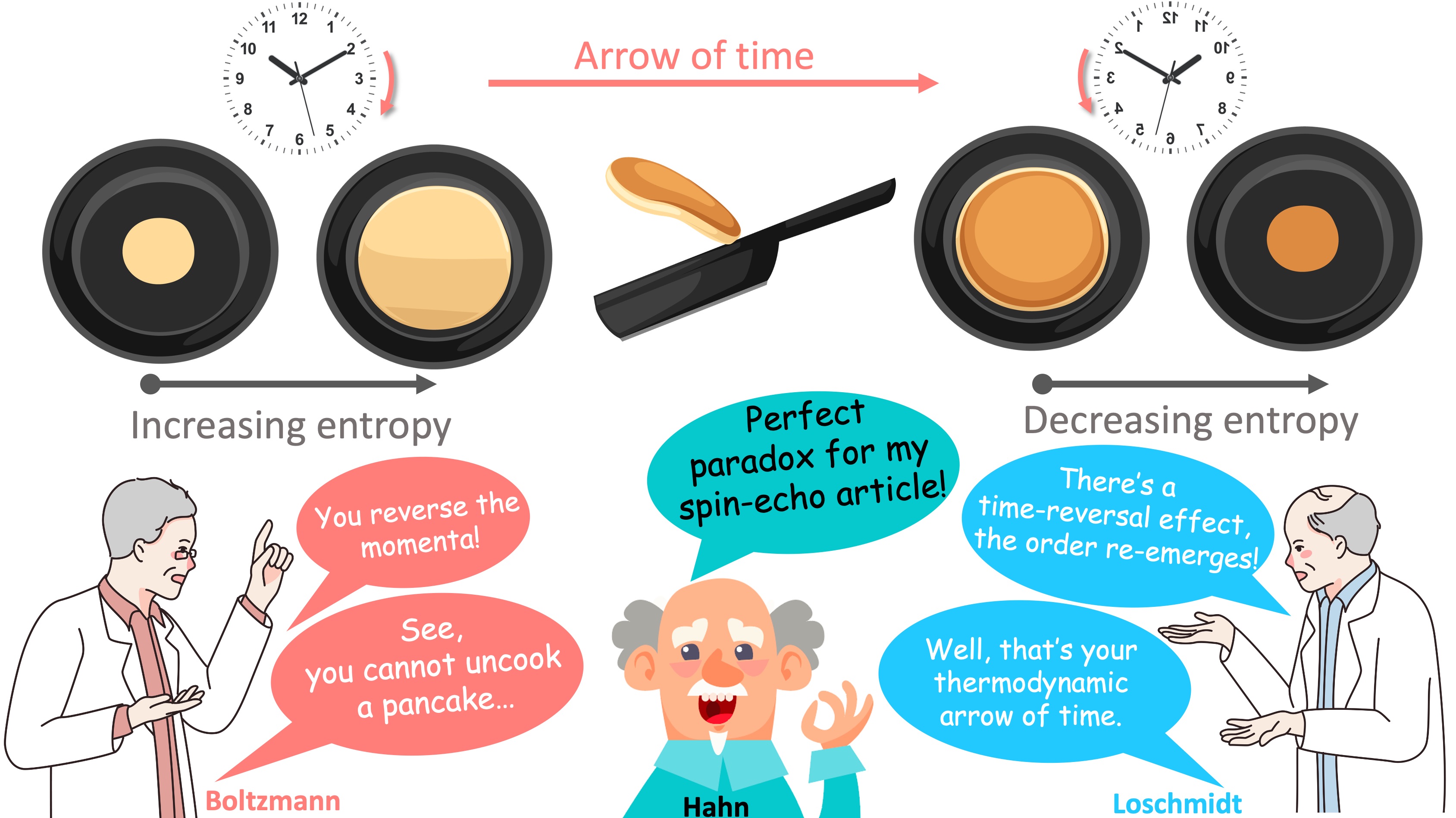
Figure 15:The second law of the thermodynamics (Boltzmann) vs the time reversal symmetry (Loschmidt) and the relation of this conflict to spin-echo (Hahn). The pancake analogy is followed in Figure 16 for completeness.
Following an excitation pulse, the spin pool goes towards disorderliness and the transverse magnetization decays (the pancake batter expands, Figure 15). In their article, Brewer and Hahn discuss resurfacing of an ordered state out of this increasing entropy by reversing the phase order of the spins (the cooked pancake contracts). By retaining the pancake analogy, Figure 16 simulates a spin-echo (SE) pulse sequence and shows the spin evolution at certain time points. At the point (B), a 90°excitation pulse rotates the net magnetization to transfer plane, and after some time, the spins dephase (C, arrows fanning out in the x-y spin scatter plot) as the FID disappears. The “refocusing pulse” rotates the net magnetization by 180°in the transverse plane (D) and reverses the phase order of the spins, analogous to flipping the pancake (Figure 16). After a period equal to the duration between the 90°and 180°RF pulses, a spin echo is formed (F). The time elapses between the center of the excitation pulse and the peak of the echo signal is termed the echo time (TE).
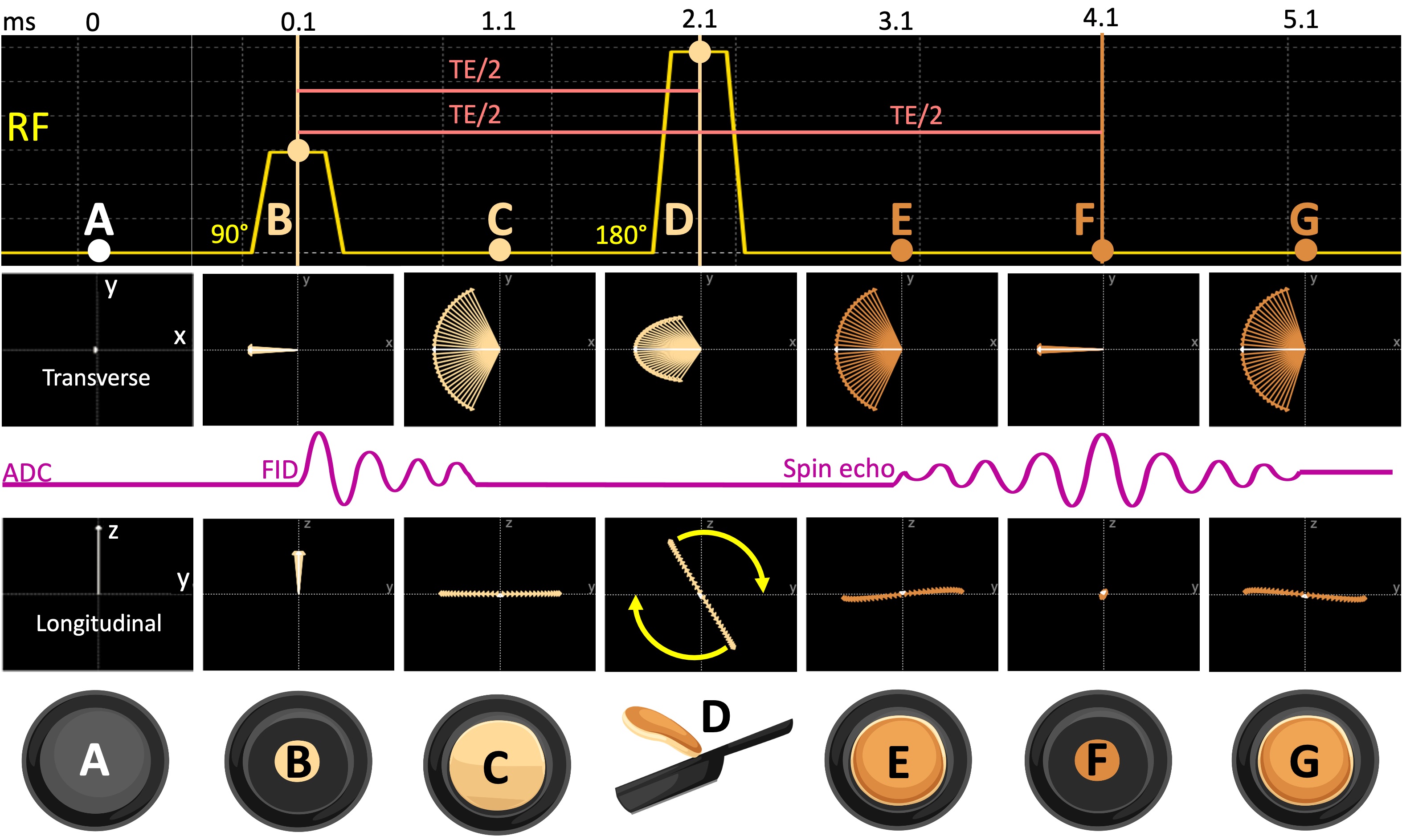
Figure 16:The spin evolution diagram of a spin-echo sequence is shown (A) before the excitation, (B) at the peak of the excitation pulse, (C) one millisecond after the 90°pulse, (D) at the peak of the refocusing pulse, (E) one millisecond after the 180°pulse, (F) at the echo time (TE) and (G) following the echo.
Equation Eq. 4 shows the signal representation of a standard SE acquisition. Given that the brightness of the image pixels is determined by the magnitude of the signal S, the relevant contribution of T1 and T2 to the image contrast can be adjusted by changing the TR and TE. For TE → 0 (i.e. short TE), the last term of the equation converges to identity, reducing the T2 contribution. If this is coiled with a long TR (TR → inf), the exponential in the second term of the equation converges to zero, reducing the T1 contribution. Therefore when the TE is short and the TR is long, the contribution to image contrast comes from the density of the spins, i.e. proton density. On the other hand, to increase the T2-weighting by keeping TR the same (long), the TE must be increased (the importance of the last term increases). Figure 17 exemplifies this by showing the same image across 6 echoes, where substances with longer T2 (e.g., eyes and the cerebrospinal fluid (CSF)) appear gradually brighter compared to the other structures in the image as the TE increases.
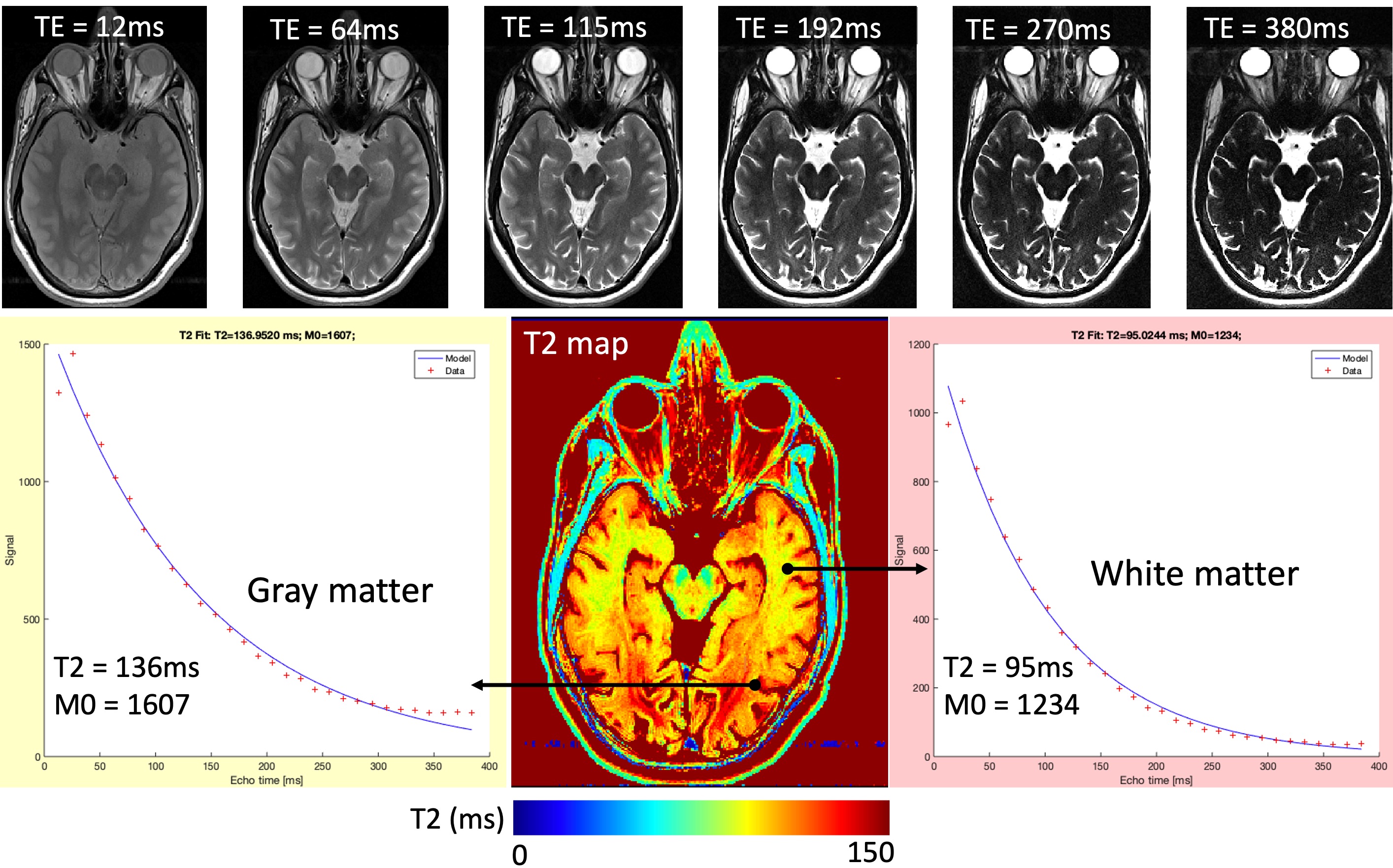
Figure 17:An example T2 map, estimated by fitting voxel-wise brightness values (red plus signs) across 32 echo times to the exponential decay (blue line) defined by Equation Eq. 4. The top row shows how conventional image contrast changes from proton-density to T2-weighted as the TE increases from 12ms to 380ms.
Since the signal representation is known for the basic SE acquisition, the signal (the voxel brightness) can be sampled at several TE’s and fitted to the exponential decay defined by the last term of the equation to calculate T2, namely T2 mapping. The second term of the equation will not be taken into account, as the TR will be kept constant across the samples. Figure 17 shows a T2 mapping example, where an axial image of the human brain was collected across 32 TE’s ranging from 12 to 380ms.
So far we looked at how an echo forms out of a 90-180° pulse pair, and created a T2 map based on its signal representation. Although the images created using SE convey good soft-tissue contrast and are robust against motion artifacts, they often come at the cost of long acquisition time (TR ranges from half to a few seconds) and high RF energy deposition.
4.0.2Gradient Echo and T1 mapping
Fortunately, MRI offers yet another way to generate echoes by taking advantage of the FID following a single RF pulse. The reversal effect needed for echoing the signal is achieved by dephasing and rephasing the spins with the use of a bipolar gradient (Figure 18). Therefore, this method is named the gradient echo (GRE).
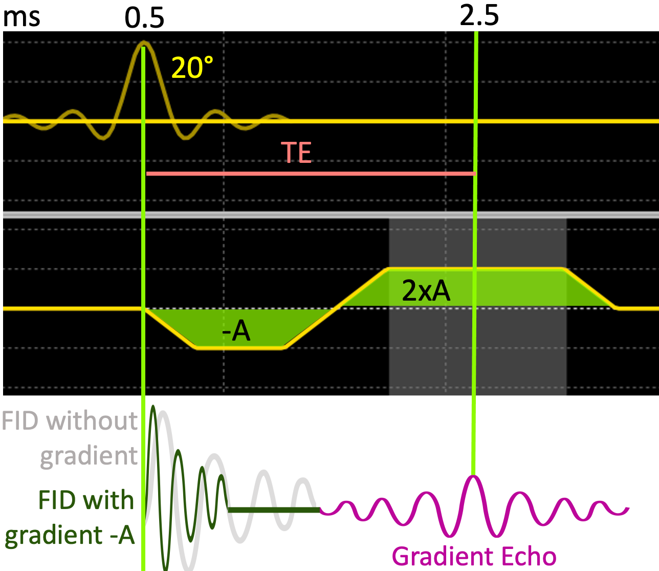
Figure 18:The formation of gradient echo by playing a bipolar gradient followed by a 20°RF pulse.
Unlike SE-based sequences, GRE sequences allow for shorter TE (a few milliseconds) and TR (10-50 milliseconds), resulting in faster acquisitions. In conventional imaging, one of the most popular GRE sequences is the spoiled gradient-echo (SPGR) sequence (Haase et al., 1986), as it allows large volumetric coverage within clinically feasible scan durations. SPGR is also widely used as a basis for various qMRI methods, because it provides a simple signal representation:
Unlike the SE signal representation (Equation Eq. 4), Equation Eq. 5 does not include a term explaining the decay of the transverse magnetization by T2. Instead, the last term of the SPGR signal representation indicates that the TE governs the signal contribution of – the effective T2. As the GRE is restored from the FID (Figure 18), the resulting echo is susceptible to slight variations in the main magnetic field. These variations may originate from the hardware-related imperfections of the B0, or from the field disruptions induced by adjacent substances with distinct magnetization levels, such as the air-tissue interfaces around the nasal cavity. As a result, T2 weighting cannot be achieved with SPGR. Instead, the second term of the Equation 2.5 indicates that the SPGR sequence is primarily T1- weighted, which can be controlled by changing the flip angle (FA) of the excitation pulse () or the TR.
After a number of GRE excitation pulses, the longitudinal magnetization reaches a dynamic equilibrium, i.e. steady-state. When the steady state is reached, the spin system looks static to the observations at a macro-scale, whereas the underlying spin interactions carry on by balancing out each other. This is similar to a person walking up (T1 recovery) an escalator that is going down (the excitation pulse). When this equilibrium is accounted for by the Equation Eq. 5, the FA that maximizes the signal for a fixed TR is given by:
where is known as the Ernst Angle (Ernst and Anderson, 1966). Figure 19 shows this relationship by simulating an SPGR signal across multiple FA at a fixed TR of 30ms for a substance with T1=800ms. It can be seen that the signal is maximized around an FA of 15°, as given by the Equation Eq. 6 for these settings (Figure 19).
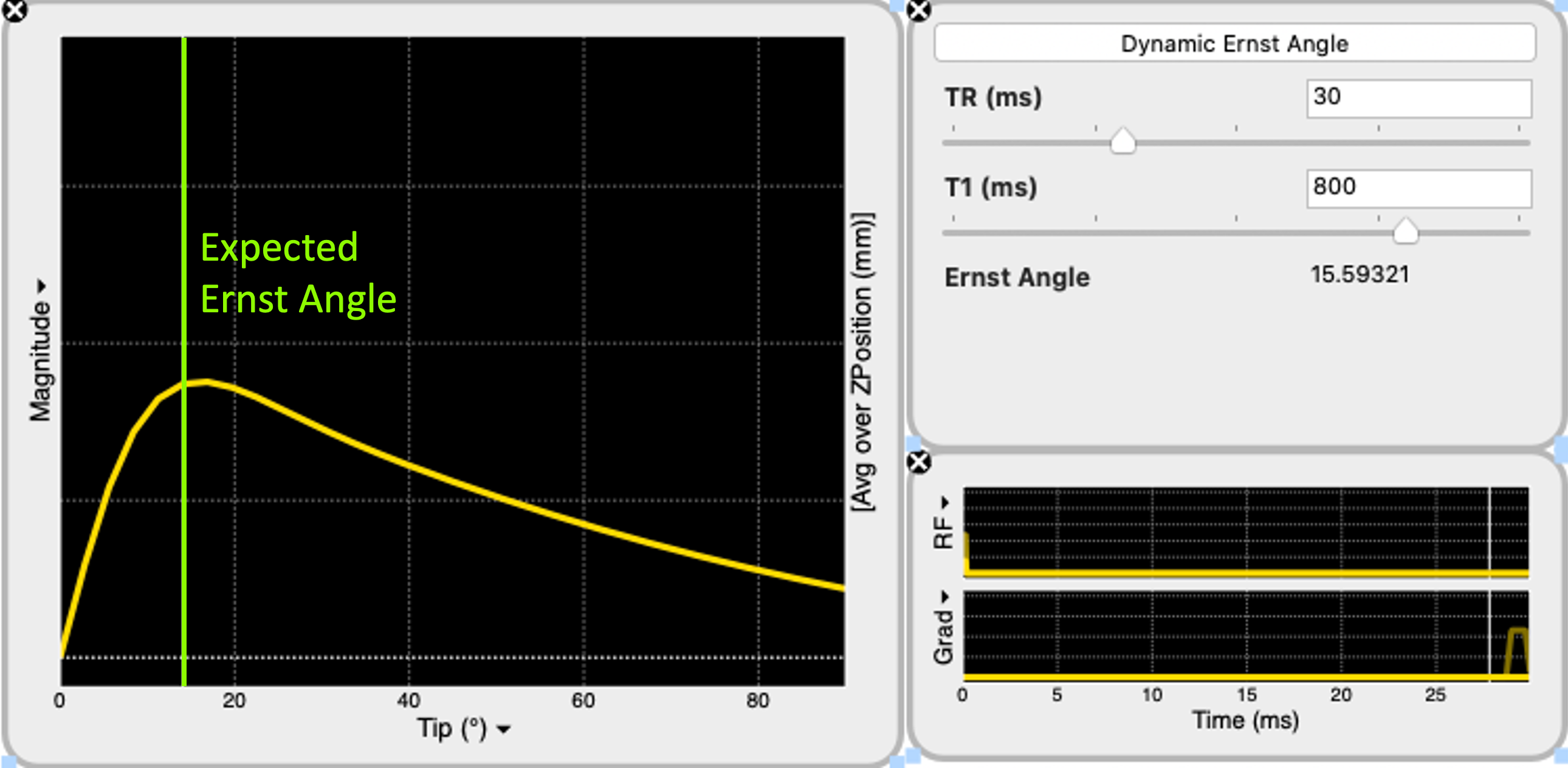
Figure 19:Spoiled gradient-echo (SPGR) signal is simulated for excitation flip angle (FA) ranging from 0 to 90°. With the repetition time set to 30ms, the Ernst Angle () is calculated at 16°for a spin system with T1 of 800ms (Equation Eq. 6). The simulated signal agrees with the calculation, indicating that the signal is the highest when the FA is around 16°(green line).
However, this relationship is valid under the assumption that the transverse magnetization is zero. Therefore, any residual transverse magnetization during the readout violates the steady-state conditions of the signal representation given by Equation Eq. 6. To avoid this, the entire spin system is dephased at the end of each TR by using a spoiler gradient, hence the name the “spoiled” GRE. In real-world pulse sequence implementations, the gradient spoiling is coupled with RF spoiling by phase cycling the excitation from TR to TR at predetermined increments (Zur et al., 1991). Figure 20 displays Bloch simulation results, indicating the critical role of selecting the spoiler gradient area (a), enabling RF spoiling (b) and the selection of a proper phase increment value in disrupting the residual transverse magnetization. The effect of spoiling efficiency becomes particularly important when multiple SPGR acquisitions are performed at different flip angles to calculate a T1 map, namely variable flip angle (VFA) method (Fram et al., 1987). This is simply because when the observed data deviates from the expected signal representation (Figure 20), the fitted parameters become inaccurate. A more theoretical explanation of the VFA T1 mapping method, its accuracy aspects and limitations are explained in the T1 mapping chapter of this MOOC.
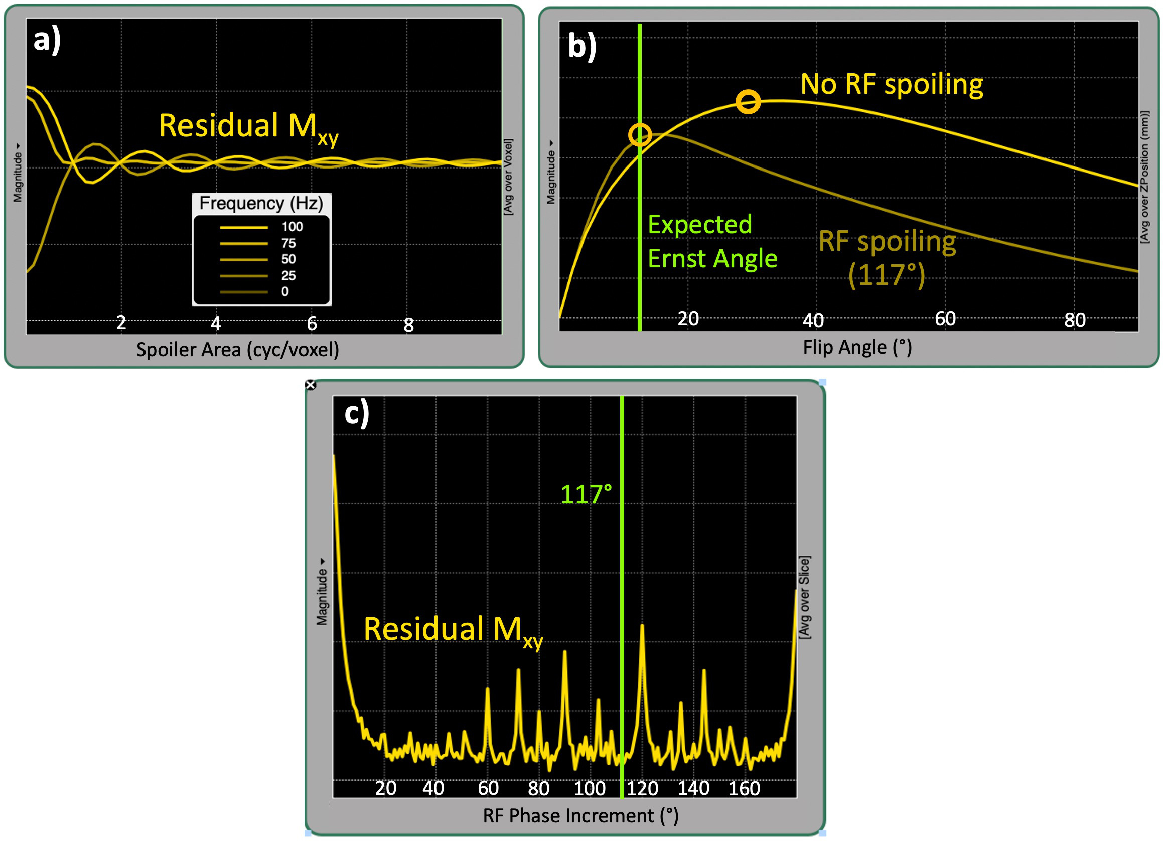
Figure 20:The influence of spoiling on SPGR signal is simulated for (a) the spoiling gradient area ranging from 0 to 10 (cyc/voxel), (b) enabling/disabling RF spoiling at 117° quadratic phase increment and (c) different phase increment values ranging from 0 to 180°.
Figure 21 shows an example T1 mapping application using the SPGR sequence in a phantom with known values. The acquisitions were performed at two flip angles of 20° (a) and 6° (b), and TR=32ms. Both images show the center of a plate accommodating 14 spheres with T1 values ranging from 0.1 to 1.99 seconds in clockwise ascending order (R1 to R10). In agreement with the Equation 2.4, the image acquired at the higher FA shows superior T1 contrast (a), as the pixel brightness varies inversely with the reference T1 values (d). On the other hand, spheres in the lower FA image show similar brightness (b), in proportion with the spin density of the spheres. From this image pair, a T1 map (c) was estimated using a linear fit as described in the VFA section of this book, exhibiting good accuracy across the reference values.
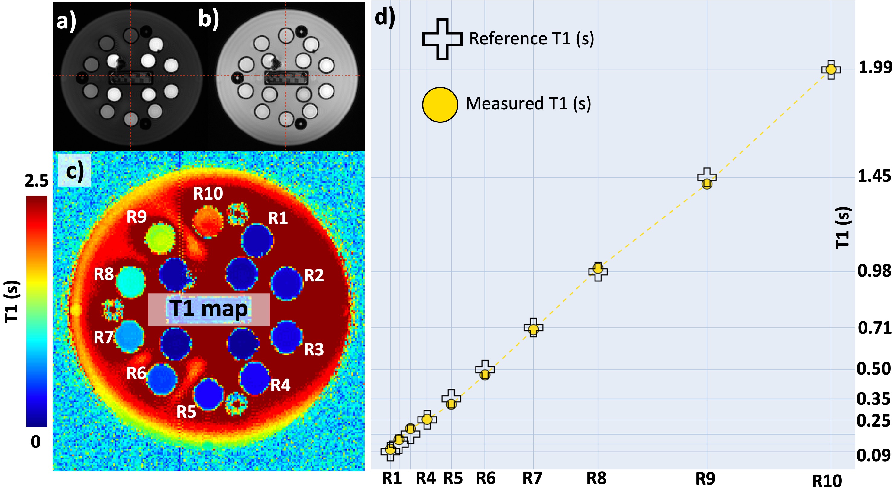
Figure 21:Variable flip angle (VFA) using SPGR sequence. a) T1-weighted and b) PD- weighted images of ISMRM/NIST system phantom acquired at 18 and 32ms, respectively. c) T1 map estimated by fitting images (a) and (b) to the relaxational component of the Equation 2.5. d) The comparison of the estimated and reference T1 values.
In this section, we covered two fundamental pulse sequences: SE and SPGR. Starting from spin-level interactions, we looked at the signal representations of each sequence and how acquisition parameters are associated with the contrast characteristics of the resulting conventional images. By doing so, we analyzed how pixel brightness emerges from two values, T2 and T1. Then using the same signal representations, we came full circle back (in case you were wondering what it meant) to these values from the pixel brightness by applying two fundamental qMRI methods, multi-echo SE for T2 and VFA for T1 mapping. A more entertaining summary of the SE and GRE sequences is unintentionally delivered by two indie rock albums (Figure 22).

Figure 22:Two (slightly modified) album covers by the Artic Monkeys and the Districts summarizing spin-echo (SE) and spoiled gradient-echo (SPGR) sequences.
5Will qMRI take over the world?
If qMRI is possible and powerful, why is clinical imaging still conventional?
“The court found that Fonar failed to establish the existence of standard T1 and T2 values, which are limitations of the asserted claims...” (GE vs Fonar 1996, U.S. Fed. Cir.)
This is partly because of the inherently complex make-up of the human body, where sensitivity alone is not enough to tease out biological variability. Quantifications should also be specific to the targeted microstructure, such as the myelin in the living human brain. For this purpose alone, the literature offers more than 30 methods for quantifying myelin at varying methodological complexity, yet they all appear to be statistically indistinguishable in specifying myelin (Mancini et al., 2020). This indicates that a lack of methodological extensity is not the culprit preventing qMRI from clinical use. Quite the contrary, there is an abundance of solutions, yet we cannot make an informed decision about which method to use. This problem has multiple roots and Figure 23 outlines the components of a qMRI study for identifying them.

Figure 23:An illustration of the components that make up a qMRI study.
5.1Vendor-native differences challenge the reliability of qMRI
Every qMRI study starts with the acquisition of a set of conventional images. This is often achieved by altering protocol parameters according to the signal representation of the respective pulse sequence, i.e. successive runs. As previously shown in the SPGR example for T1 mapping (Figure 20), there are various parameters that are vital to the measurement accuracy and precision. In general, strict metrological standards are established for the manufacturing process of any medical device expected to fulfill some accuracy requirements. For example, all the ventilator vendors are obliged to disclose their measurement uncertainty for inspiratory oxygen concentration (ISO 80601-2-12:2011). However, MRI is exempt from such a class of essential performance assessments on the accuracy and precision, given that the medical diagnoses using conventional MRI depend on qualitative feature recognition (Figure 1). In turn, design considerations that matter to the reliability of qMRI measurements fall through the cracks of the device manufacturing and programming processes. Although this is understandable from a vendor’s cost-effectiveness standpoint, it bears dire consequences on the quantitative applications.
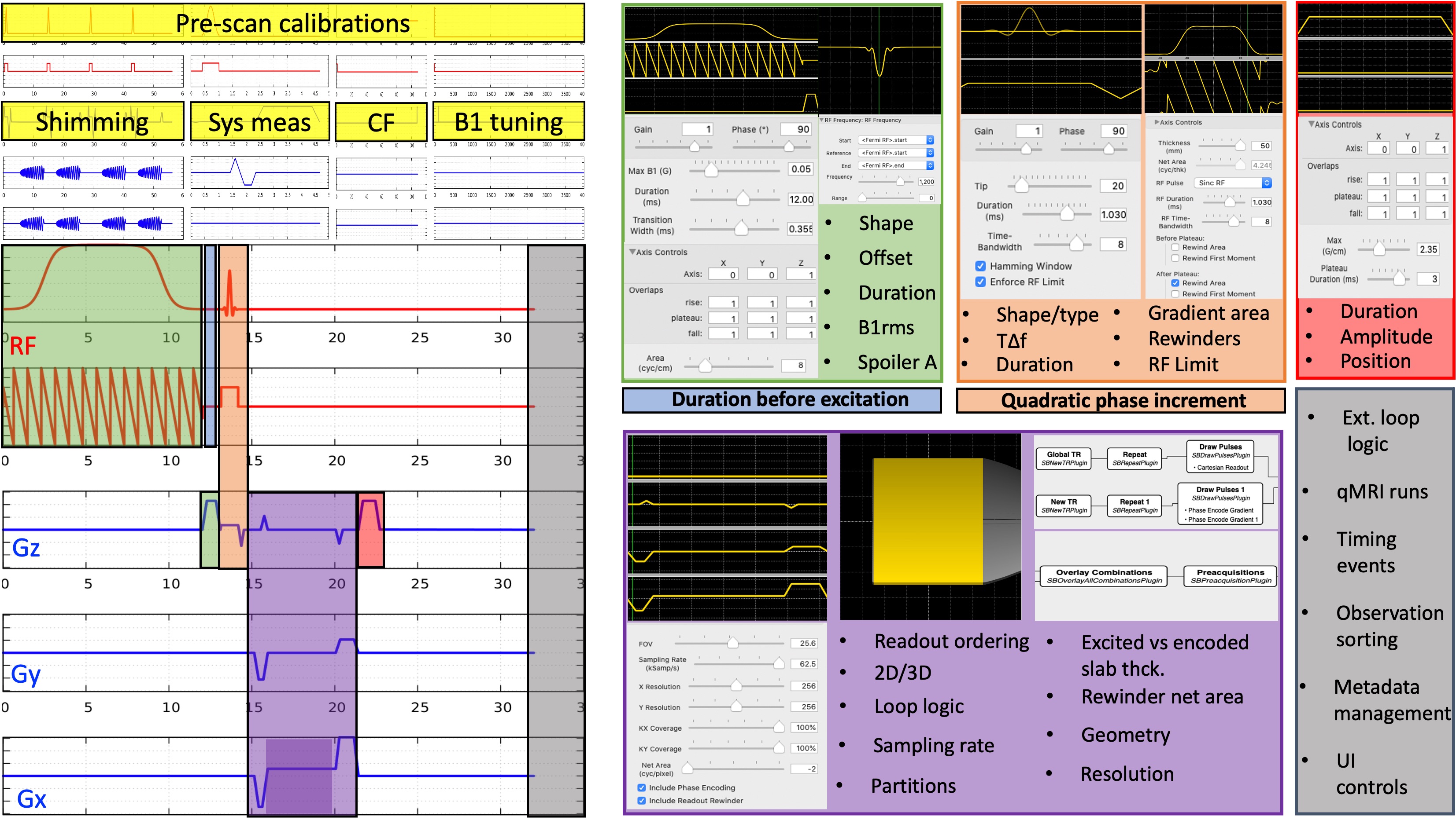
Figure 24:Choices involved in the implementation of a magnetization-transfer weighted spoiled gradient echo (SPGR) sequence are shown for all the gradient and RF waveforms involved.
Even for the simplest sequence implementations, there may be several parameters that matter to quantification, but are hidden from the end user. Figure 24 shows the implementation- level parameters that are available after the type/shape selections were made for an SPGR sequence with a magnetization-transfer saturation pulse. In addition to the sequence itself, pre-scan calibrations such as shimming, center frequency tuning and transmit gain adjustments are other factors that affect the measurement accuracy. For example, neither of the major vendor implementations enable the selection of spoiling gradient area (FFigure 20a), RF spoiling regime (Figure 20b,c), magnetization transfer (MT) pulse specifications, ex- citation pulse type or the ordering of the observations (Figure 24). The more advanced the sequence, the more implementation choices come to the surface. These restrictions and unknowns brought by vendor-specific sequence implementations trap tens of qMRI measurements into a maze of variability and prevent them from reaching the clinics (Figure 25).
After the raw data is acquired, it has to be reconstructed to generate images, which is yet another process with a wide range of options to choose from. Therefore, properly formatting and making the raw data accessible is a non-trivial interim step for the provenance of the following steps. In addition, the relationship between the reconstructed images and the grouping logic entailed by the qMRI model should be retained along with sufficient metadata. Even though there is an emerging data standard for organizing the raw data (Inati et al., 2017), there is not a community consensus on how to organize qMRI datasets (Figure 23). This creates idiosyncrasies, challenging interoperability and decreasing efficiency of processing qMRI data.
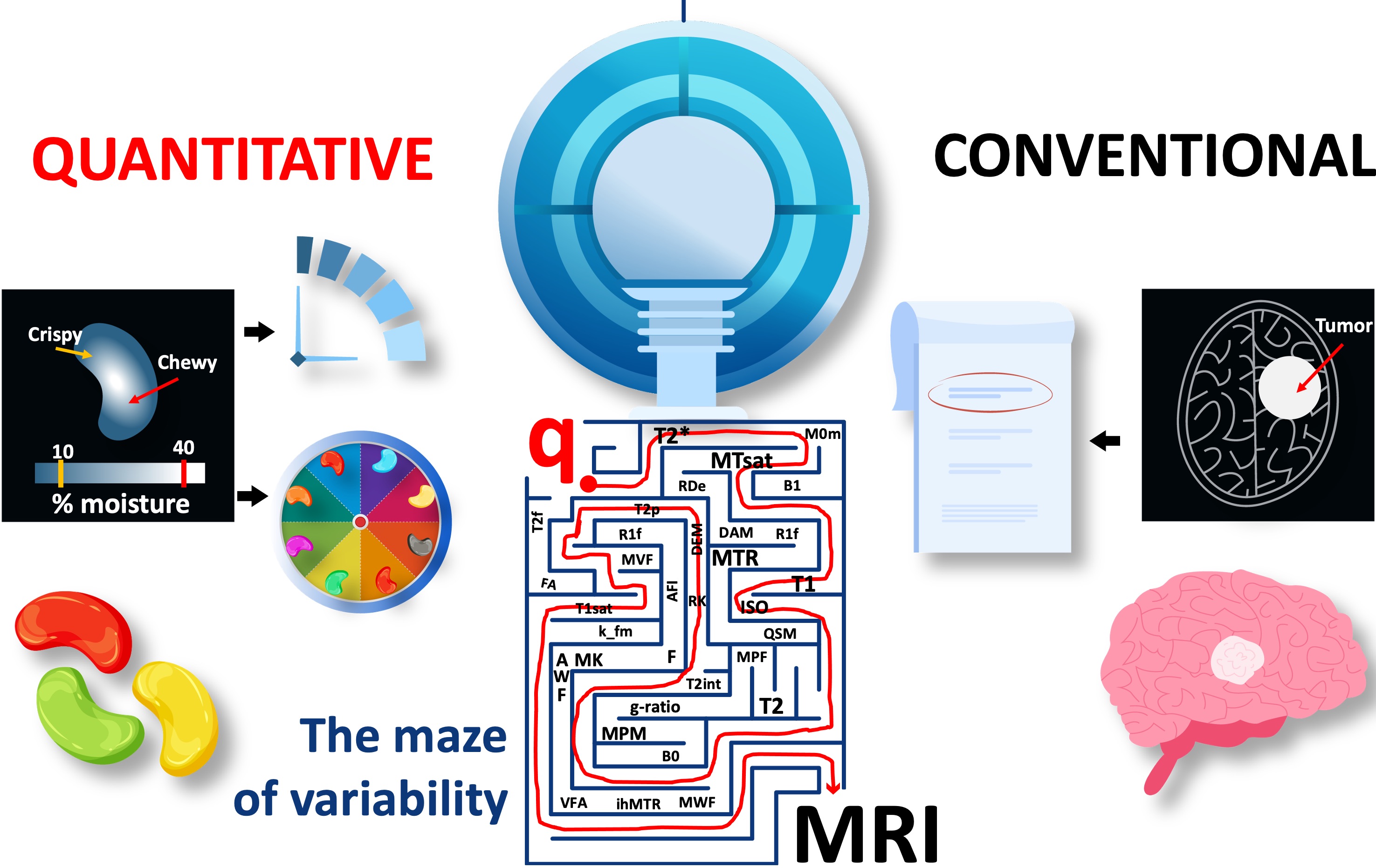
Figure 25:The current landscape of quantitative MRI is a maze of variability for amazing methods. A complete recipe is needed to chart out the path towards clinics.
There are dozens of publications introducing new qMRI methods, yet a majority of these implementations are kept within their labs of origin, making it challenging to reproduce qMRI studies. This is partly caused by the vendor restrictions. Nonetheless, it is generally possible to share the workflow components of the developed methods. Figure 23 shows that all qMRI methods share a common methodology at their core: a signal representation (qRecipe) that relates a set of parametrically linked MR images (qData) to some microstructural and physical features (qMap) by computation (qProcessing). Although these ingrained attributes exist at a conceptual level in the source code developed by independent developers, there is not a consensus on how to represent them in a programming paradigm. Even though 80% of the source code made available by the MRI developers share the same programming language (MATLAB) (Boudreau, 2019), there is still a need for a common framework for the development of qMRI methods in MATLAB to make implementations easier.
To summarize the problems mentioned above, there are three outstanding issues that hinder the standardization of qMRI:
Most methods are developed using in-house code that is difficult to distribute, challenging the accessibility and reproducibility of qMRI studies.
The lack of a qMRI data standard poses an interoperability challenge for open-source solutions aiming at making qMRI methods publicly accessible.
The unknowns involved in the implementation of commercial pulse sequences constitute a substantial source of (vendor-specific) variability in fitting quantitative parameters using voxel brightness data.
5.2Vendor-neutral qMRI and its importance
--MISSING--
- Nishimura, D. G. (1996). Principles of magnetic resonance imaging. Stanford University.
- Troutman, M. Y., Mastikhin, I. V., Balcom, B. J., Eads, T. M., & Ziegler, G. R. (2001). Moisture migration in soft-panned confections during engrossing and aging as observed by magnetic resonance imaging. Journal of Food Engineering, 48(3), 257–267.
- Ziegler, G. R., MacMillan, B., & Balcom, B. J. (2003). Moisture migration in starch molding operations as observed by magnetic resonance imaging. Food Research International, 36(4), 331–340.
- Mariette, F., Collewet, G., Davenel, A., Lucas, T., & Musse, M. (2012). Quantitative MRI in food science & food engineering. Encyclopedia of Magnetic Resonance by John Wiley.
- Gambon, D. (2015). The Crazy World of Candy. Tandartspraktijk, 36(7), 17–23.
- Dreizen, P. (2004). The Nobel prize for MRI: a wonderful discovery and a sad controversy. The Lancet, 363(9402), 78.
- Damadian, R. (1971). Tumor detection by nuclear magnetic resonance. Science, 171(3976), 1151–1153.
- Damadian, R. (1974). Apparatus and method for detecting cancer in tissue (US3789832A). https://patents.google.com/patent/US3789832?oq=damadian+1971
- Lauterbur, P. C. (1989). Image formation by induced local interactions. Examples employing nuclear magnetic resonance. 1973 [Journal Article]. Clin Orthop Relat Res, 244, 3–6. https://www.ncbi.nlm.nih.gov/pubmed/2663289
- Dawson, M. J. (2013). Paul Lauterbur and the Invention of MRI. MIT Press.
- Turner, R. (2017). Peter Mansfield (1933–2017). Nature, 543(7644), 180–180. 10.1038/543180a
- Mansfield, P., & Maudsley, A. A. (1977). Planar spin imaging by NMR. Journal of Magnetic Resonance (1969), 27(1), 101–119. https://doi.org/10.1016/0022-2364(77)90197-4
- Harris, R. F. (2003). Nobel grudge. Current Biology, 13(22), R857.
- Tamir, J. I., Ong, F., Anand, S., Karasan, E., Wang, K., & Lustig, M. (2020). Computational MRI With Physics-Based Constraints: Application to Multicontrast and Quantitative Imaging. IEEE Signal Processing Magazine, 37(1), 94–104. 10.1109/msp.2019.2940062