1Introduction
T1, or spin-lattice relaxation time, is a fundamental magnetic resonance property that characterizes the rate at which excited nuclear spins return to equilibrium with their surrounding environment. Beyond its value as a quantitative biomarker, accurate T1 knowledge is essential for optimizing imaging protocols, such as computing the Ernst angle for maximum signal-to-noise ratio in spoiled gradient echo sequences Ernst & Anderson, 1966. T1 values also serve as important correction factors in other quantitative MRI techniques, including quantitative magnetization transfer imaging Cercignani et al., 2005Yarnykh, 2002 and dynamic contrast enhanced imaging Li et al., 2018Sung et al., 2013, making T1 mapping a crucial component of comprehensive quantitative MRI protocols.
This chapter explores three principal methodologies for quantitative T1 mapping, each with distinct advantages and limitations. The inversion recovery technique, widely considered the gold standard Stikov et al., 2015, provides robust T1 estimates through direct sampling of the longitudinal magnetization recovery curve following an inversion pulse. Despite its proven accuracy, conventional implementations require long repetition times on the order of 2-5 T1 Steen et al., 1994, making whole-organ mapping challenging within clinically feasible times. In contrast, variable flip angle (VFA) methods offer rapid 3D T1 mapping capabilities through acquisition of multiple spoiled gradient echo images with different excitation angles Christensen et al., 1974Fram et al., 1987Gupta, 1977. While significantly faster than inversion recovery, VFA techniques demonstrate heightened sensitivity to flip angle inaccuracies resulting from transmit field inhomogeneities, necessitating additional B1 mapping for correction Sled & Pike, 1998Boudreau et al., 2017.
More recently, dictionary-based approaches like MP2RAGE have emerged that combine elements of both inversion recovery and variable flip angle methodologies Marques et al., 2010. These techniques leverage pre-calculated signal dictionaries to enable rapid quantitative mapping with built-in correction for certain field inhomogeneities. The growing availability of such turnkey sequences on clinical scanners has made quantitative T1 mapping increasingly accessible for routine applications. Throughout this chapter, we will examine the theoretical foundations, practical implementations, and relative strengths of each approach, providing readers with comprehensive understanding of modern T1 mapping techniques.
2Inversion Recovery T1 Mapping
Widely considered the gold standard for T1 mapping, the inversion recovery technique estimates T1 values by fitting the signal recovery curve acquired at different delays after an inversion pulse (180°). In a typical inversion recovery experiment (Figure 2.1), the magnetization at thermal equilibrium is inverted using a 180° RF pulse. After the longitudinal magnetization recovers through spin-lattice relaxation for predetermined delay (inversion time, TI), a 90° excitation pulse is applied, followed by a readout imaging sequence (typically a spin-echo or gradient-echo readout) to create a snapshot of the longitudinal magnetization state at that TI.
Inversion recovery was first developed for NMR in the 1940s Hahn, 1949Drain, 1949, and the first T1 map was acquired using a saturation-recovery technique (90° as a preparation pulse instead of 180°) by Pykett & Mansfield, 1978. Some distinct advantages of inversion recovery are its large dynamic range of signal change and an insensitivity to pulse sequence parameter imperfections Stikov et al., 2015. Despite its proven robustness at measuring T1, inversion recovery is scarcely used in practice, because conventional implementations require repetition times (TRs) on the order of 2 to 5 T1 Steen et al., 1994, making it challenging to acquire whole-organ T1 maps in a clinically feasible time. Nonetheless, it is continuously used as a reference measurement during the development of new techniques, or when comparing different T1 mapping techniques, and several variations of the inversion recovery technique have been developed, making it practical for some applications Messroghli et al., 2004Piechnik et al., 2010.

Figure 2.1:Pulse sequence of an inversion recovery experiment.
Signal Modelling
The steady-state longitudinal magnetization of an inversion recovery experiment can be derived from the Bloch equations for the pulse sequence \theta_{180} – TI – – (TR-TI)}, and is given by:
where is the longitudinal magnetization prior to the pulse. If the in-phase real signal is desired, it can be calculated by multiplying Eq. 2.1 by , where is a constant. This general equation can be simplified by grouping together the constants for each measurements regardless of their values (i.e. at each TI, same TE and are used) and assuming an ideal inversion pulse:
where the first three terms and the denominator of Eq. 2.1 have been grouped together into the constant . If the experiment is designed such that TR is long enough to allow for full relaxation of the magnetization (TR > 5 T1), we can do an additional approximation by dropping the last term in Eq. 2.2:
The simplicity of the signal model described by Eq. 2.3, both in its equation and experimental implementation, has made it the most widely used equation to describe the signal evolution in an inversion recovery T1 mapping experiment. The magnetization curves are plotted in Figure 2.2 for approximate T1 values of three different tissues in the brain. Note that in many practical implementations, magnitude-only images are acquired, so the signal measured would be proportional to the absolute value of Eq. 2.3.
Figure 2.2:Inversion recovery curves (Eq. 2.2) for three different T1 values, approximating the main types of tissue in the brain.
Practically, Eq. 2.1 is the better choice for simulating the signal of an inversion recovery experiment, as the TRs are often chosen to be greater than 5 T1 of the tissue-of-interest, which rarely coincides with the longest T1 present (e.g. TR may be sufficiently long for white matter, but not for CSF which could also be present in the volume). Eq. 2.3 also assumes ideal inversion pulses, which is rarely the case due to slice profile effects. Figure 2.3 displays the inversion recovery signal magnitude (complete relaxation normalized to 1) of an experiment with TR = 5 s and T1 values ranging between 250 ms to 5 s, calculated using both equations.
Figure 2.3:Signal recovery curves simulated using Eq. 2.3 (solid) and Eq. 2.1 (dotted) with a TR = 5 s for T1 values ranging between 0.25 to 5 s.
Click here to view the qMRLab (MATLAB/Octave) code that generated Figure 2.2.
% Verbosity level 0 overrides the disp function and supresses warnings.
% Once executed, they cannot be restored in this session
% (kernel needs to be restarted or a new notebook opened.)
VERBOSITY_LEVEL = 0;

if VERBOSITY_LEVEL==0
    % This hack was used to supress outputs from external tools
    % in the Jupyter Book.
    function disp(x)
    end
    warning('off','all')
end

try
    cd qMRLab
catch
    try
        cd ../../../qMRLab
    catch
        cd ../qMRLab
    end
end

startup
clear all

%% Setup parameters
% All times are in seconds
% All flip angles are in degrees

params.TR = 5.0;
params.TI = linspace(0.001, params.TR, 1000);

params.TE = 0.004;
params.T2 = 0.040;

params.EXC_FA = 90;  % Excitation flip angle
params.INV_FA = 180; % Inversion flip angle

params.signalConstant = 1;

%% Calculate signals
%
% The option 'GRE-IR' selects the analytical equations for the
% gradient echo readout inversion recovery experiment The option
% '4' is a flag that selects the long TR approximation of the
% analytical solution (TR>>T1), Eq. 3 of the blog post.
%
% To see all the options available, run:
% `help inversion_recovery.analytical_solution`

% White matter
params.T1 = 0.900; % in seconds

signal_WM = inversion_recovery.analytical_solution(params, 'GRE-IR', 4);

% Grey matter
params.T1 = 1.500;  % in seconds
signal_GM = inversion_recovery.analytical_solution(params, 'GRE-IR', 4);

% CSF
params.T1 = 4.000;  % in seconds
signal_CSF = inversion_recovery.analytical_solution(params, 'GRE-IR', 4);
Click here to view the qMRLab (MATLAB/Octave) code that generated Figure 2.3.
% Verbosity level 0 overrides the disp function and supresses warnings.
% Once executed, they cannot be restored in this session
% (kernel needs to be restarted or a new notebook opened.)
VERBOSITY_LEVEL = 0;

if VERBOSITY_LEVEL==0
    % This hack was used to supress outputs from external tools
    % in the Jupyter Book.
    function disp(x)
    end
    warning('off','all')
end

try
    cd qMRLab
catch
    try
        cd ../../../qMRLab
    catch
        cd ../qMRLab
    end
end

startup
clear all

%% Setup parameters
% All times are in seconds
% All flip angles are in degrees

params.TR = 5.0;
params.TI = linspace(0.001, params.TR, 1000);

params.TE = 0.004;
params.T2 = 0.040;

params.EXC_FA = 90;  % Excitation flip angle
params.INV_FA = 180; % Inversion flip angle

params.signalConstant = 1;

T1_range = 0.25:0.25:5; % in seconds

%% Calculate signals
%
% The option 'GRE-IR' selects the analytical equations for the
% gradient echo readout inversion recovery experiment. The option
% '1' is a flag that selects full analytical solution equation
% (no approximation), Eq. 1 of the blog post. The option '4' is a
% flag that selects the long TR approximation of the analytical
% solution (TR>>T1), Eq. 3 of the blog post.
%
% To see all the options available, run:
% `help inversion_recovery.analytical_solution`

for ii = 1:length(T1_range)
    params.T1 = T1_range(ii);

    signal_T1_Eq1{ii} = inversion_recovery.analytical_solution(params, 'GRE-IR', 1);

    signal_T1_Eq3{ii} = inversion_recovery.analytical_solution(params, 'GRE-IR', 4);
end
Data Fitting
Several factors impact the choice of the inversion recovery fitting algorithm. If only magnitude images are available, then a polarity-inversion is often implemented to restore the non-exponential magnitude curves (Figure 2.3) into the exponential form (Figure 2.2). This process is sensitive to noise due to the Rician noise creating a non-zero level at the signal null. If phase data is also available, then a phase term must be added to the fitting equation Barral et al., 2010. Equation 2.3 must only be used to fit data for the long TR regime (TR > 5 T1), which in practice is rarely satisfied for all tissues in subjects.
Early implementations of inversion recovery fitting algorithms were designed around the computational power available at the time. These included the “null method” Pykett et al., 1983, assuming that each T1 value has unique zero-crossings (see Figure 2.2), and linear fitting of a rearranged version of Equation 2.3 on a semi-log plot Fukushima, 1981. Nowadays, a non-linear least-squares fitting algorithm (e.g. Levenberg-Marquardt) is more appropriate, and can be applied to either approximate or general forms of the signal model (Equation 2.3 or Equation 2.1). More recent work Barral et al., 2010 demonstrated that T1 maps can also be fitted much faster (up to 75 times compared to Levenberg-Marquardt) to fit Equation 2.1 – without a precision penalty – by using a reduced-dimension non-linear least-squares (RD-NLS) algorithm. It was demonstrated that the following simplified 5-parameter equation can be sufficient for accurate T1 mapping:
where and are complex values. If magnitude-only data is available, a 3-parameter model can be sufficient by taking the absolute value of Equation 2.4. While the RD-NLS algorithms are too complex to be presented here (the reader is referred to the paper, Barral et al., 2010), the code for these algorithms was released open-source along with the original publication, and is also available as a qMRLab T1 mapping model. One important thing to note about Equation 2.4 is that it is general – no assumption is made about TR – and is thus as robust as Equation 2.1 as long as all pulse sequence parameters other than TI are kept constant between each measurement. Figure 2.4 compares simulated data (Equation 2.1) using a range of TRs (1.5 T1 to 5 T1) fitted using either RD-NLS & Equation 2.4 or a Levenberg-Marquardt fit of Equation 2.2.
Figure 2.4:Fitting comparison of simulated data (blue markers) with T1 = 1 s and TR = 1.5 to 5 s, using fitted using RD-NLS & Equation 2.4 (green) and Levenberg-Marquardt & Equation 2.2 (orange, long TR approximation).
Figure 2.5 displays an example brain dataset from an inversion recovery experiment, along with the T1 map fitted using the RD-NLS technique.
Figure 2.5:Example inversion recovery dataset of a healthy adult brain (left). Inversion times used to acquire this magnitude image dataset were 30 ms, 530 ms, 1030 ms, and 1530 ms, and the TR used was 1550 ms. The T1 map (right) was fitted using a RD-NLS algorithm.
Click here to view the qMRLab (MATLAB/Octave) code that generated Figure 2.4.
% Verbosity level 0 overrides the disp function and supresses warnings.
% Once executed, they cannot be restored in this session
% (kernel needs to be restarted or a new notebook opened.)
VERBOSITY_LEVEL = 0;

if VERBOSITY_LEVEL==0
    % This hack was used to supress outputs from external tools
    % in the Jupyter Book.
    function disp(x)
    end
    warning('off','all')
end

try
    cd qMRLab
catch
    try
        cd ../../../qMRLab
    catch
        cd ../qMRLab
    end
end

startup
clear all

%% Setup parameters
% All times are in milliseconds
% All flip angles are in degrees

params.TI = 50:50:1500;
TR_range = 1500:50:5000;

params.EXC_FA = 90;
params.INV_FA = 180;

params.T1 = 1000;

%% Calculate signals
%
% The option 'GRE-IR' selects the analytical equations for the gradient echo readout inversion recovery experiment
% The option '1' is a flag that selects full analytical solution equation (no approximation), Eq. 1 of the blog post.
%
% To see all the options available, run `help inversion_recovery.analytical_solution`

for ii = 1:length(TR_range)
    params.TR = TR_range(ii);
    Mz_analytical(ii,:) = inversion_recovery.analytical_solution(params, 'GRE-IR', 1);
end

%% Fit data using Levenberg-Marquardt with the long TR approximation equation
%
% The option '4' is a flag that selects the long TR approximation of the analytical solution (TR>>T1), Eq. 3 of the blog post.
%
% To see all the options available, run `help inversion_recovery.fit_lm`


for ii=1:length(TR_range)
    fitOutput_lm{ii} = inversion_recovery.fit_lm(Mz_analytical(ii,:), params, 4);
    T1_lm(ii) = fitOutput_lm{ii}.T1;
end

%% Fit data using the RDLS method (Barral), Eq. 4 of the blog post.
%

% Create a qMRLab inversion recovery model object and load protocol values
irObj = inversion_recovery();
irObj.Prot.IRData.Mat = params.TI';

for ii=1:length(TR_range)

    data.IRData = Mz_analytical(ii,:);

    fitOutput_barral{ii} = irObj.fit(data);

    T1_barral(ii) = fitOutput_barral{ii}.T1;

end
Click here to view the qMRLab (MATLAB/Octave) code that generated Figure 2.5.
% Verbosity level 0 overrides the disp function and supresses warnings.
% Once executed, they cannot be restored in this session
% (kernel needs to be restarted or a new notebook opened.)
VERBOSITY_LEVEL = 0;

if VERBOSITY_LEVEL==0
    % This hack was used to supress outputs from external tools
    % in the Jupyter Book.
    function disp(x)
    end
    warning('off','all')
end

try
    cd qMRLab
catch
    try
        cd ../../../qMRLab
    catch
        cd ../qMRLab
    end
end

startup

clear all

%% MATLAB/OCTAVE CODE

% Load data into environment, and rotate mask to be aligned with IR data
load('data/ir_dataset/IRData.mat');
load('data/ir_dataset/IRMask.mat');

IRData = data;
Mask = imrotate(Mask,180);
clear data

% Format qMRLab inversion_recovery model parameters, and load them into the Model object
Model = inversion_recovery;
TI = [30; 530; 1030; 1530];
Model.Prot.IRData.Mat = [TI];

% Format data structure so that they may be fit by the model
data = struct();
data.IRData= double(IRData);
data.Mask= double(Mask);

FitResults = FitData(data,Model,0); % The '0' flag is so that no wait bar is shown.

% Code used to re-orient the images to make pretty figures, and to assign variables with the axis lengths.

T1_map = imrotate(FitResults.T1.*Mask,-90);
xAxis = [0:size(T1_map,2)-1];
yAxis = [0:size(T1_map,1)-1];

% Raw MRI data at different TI values
TI_0030 = imrotate(squeeze(IRData(:,:,:,1).*Mask),-90);
TI_0530 = imrotate(squeeze(IRData(:,:,:,2).*Mask),-90);
TI_1030 = imrotate(squeeze(IRData(:,:,:,3).*Mask),-90);
TI_1530 = imrotate(squeeze(IRData(:,:,:,4).*Mask),-90);
Benefits and Pitfalls
The conventional inversion recovery experiment is considered the gold standard T1 mapping technique for several reasons:
A typical protocol has a long TR value and a sufficient number of inversion times for stable fitting (typically 5 or more) covering the range [0, TR].
It offers a wide dynamic range of signals ([up to , ]), allowing a number of inversion times where high SNR is available to sample the signal recovery curve Fukushima, 1981.
T1 maps produced by inversion recovery are largely insensitive to inaccuracies in excitation flip angles and imperfect spoiling Stikov et al., 2015, as all parameters except TI are constant for each measurement and only a single acquisition is performed (at TI) during each TR.
One important protocol design consideration is to avoid acquiring at inversion times where the signal for T1 values of the tissue-of-interest is nulled, as the magnitude images at this TI time will be dominated by Rician noise which can negatively impact the fit under low SNR circumstances (Figure 2.6). Inversion recovery can also often be acquired using commonly available standard pulse sequences available on most MRI scanners by setting up a customized acquisition protocol, and does not require any additional calibration measurements. For an example, please visit the interactive preprint of the ISMRM Reproducible Research Group 2020 Challenge on inversion recovery T1 mapping Boudreau et al., 2023.
Figure 2.6:Monte Carlo simulations (mean and standard deviation (STD), blue markers) and fitted T1 values (mean and STD, red and green respectively) generated for a T1 value of 900 ms and 5 TI values linearly spaced across the TR (ranging from 1 to 5 s). A bump in T1 STD occurs near TR = 3000 ms, which coincides with the TR where the second TI is located near a null point for this T1 value.
Despite a widely acknowledged robustness for measuring accurate T1 maps, inversion recovery is not often used in studies. An important drawback of this technique is the need for long TR values, generally on the order of a few T1 for general models (e.g. Equations Eq. 2.1 and Eq. 2.4), and up to 5 T1 for long TR approximated models (Equation 2.3). It takes about to 10-25 minutes to acquire a single-slice T1 map using the inversion recovery technique, as only one TI is acquired per TR (2-5 s) and conventional cartesian gradient readout imaging acquires one phase encode line per excitation (for a total of ~100-200 phase encode lines). The long acquisition time makes it challenging to acquire whole-organ T1 maps in clinically feasible protocol times. Nonetheless, it is useful as a reference measurement for comparisons against other T1 mapping methods, or to acquire a single-slice T1 map of a tissue to get T1 estimates for optimization of other pulse sequences.
Click here to view the qMRLab (MATLAB/Octave) code that generated Figure 2.6.
% Verbosity level 0 overrides the disp function and supresses warnings.
% Once executed, they cannot be restored in this session
% (kernel needs to be restarted or a new notebook opened.)
VERBOSITY_LEVEL = 0;

if VERBOSITY_LEVEL==0
    % This hack was used to supress outputs from external tools
    % in the Jupyter Book.
    function disp(x)
    end
    warning('off','all')
end

try
    cd qMRLab
catch
    try
        cd ../../../qMRLab
    catch
        cd ../qMRLab
    end
end

startup
clear all

%% Setup parameters
% All times are in seconds
% All flip angles are in degrees

TR_range = 1000:100:5000; % in seconds

x = struct;
x.T1 = 900; % in seconds

Opt.SNR = 25;
Opt.M0 = 1;
Opt.FAexcite = 90; % Excitation flip angle
Opt.FAinv = 180;   % Inversion flip angle

%% Monte Carlo data simulation
% Simulate noisy signal data 1,000 time, fit the data, then calculate the means and standard deviations of the data and fitted T1
% Data is calculated by calculating the a and b values of Eq. 4 from the full analytical equations (Eq. 1)

Model = inversion_recovery;

for ii = 1:length(TR_range)
    Opt.TR = TR_range(ii);
    Opt.T1 = x.T1;
    TI_lowres(ii,:) = linspace(0.05, Opt.TR, 6)';
    Model.Prot.IRData.Mat = [TI_lowres(ii,:)];
    [ra,rb] = Model.ComputeRaRb(x,Opt);
    x.rb = rb;
    x.ra = ra;
    for jj = 1:1000
        [FitResult{ii,jj}, noisyData{ii,jj}] = Model.Sim_Single_Voxel_Curve(x,Opt,0);
        fittedT1(ii,jj) = FitResult{ii,jj}.T1;
        noisyData_array(ii,jj,:) = noisyData{ii,jj}.IRData;
    end

    for kk=1:length(TI_lowres(ii,:))
        data_mean(ii,kk) = mean(noisyData_array(ii,:,kk));
        data_std(ii,kk) = std(noisyData_array(ii,:,kk));
    end

    T1_mean(ii) = mean(fittedT1(ii,:));
    T1_std(ii) = std(fittedT1(ii,:));
end

%% Calculate the noiseless data at a higher TI resolution to plot the ideal signal curve.
%

for ii = 1:length(TR_range)
    TI_highres(ii,:) = linspace(0.05, TR_range(ii), 500);
    Model.Prot.IRData.Mat = [TI_highres(ii,:)];
    Opt.TR = TR_range(ii);
    Opt.T1 = x.T1;
    [ra,rb] = Model.ComputeRaRb(x,Opt);
    x.rb = rb;
    x.ra = ra;

    data_noiseless(ii,:) = Model.equation(x);
end
Other Saturation-Recovery T1 Mapping techniques
Several variations of the inversion recovery pulse sequence were developed to overcome challenges like those specified above. Amongst them, the Look-Locker technique Look & Locker, 1970 stands out as one of the most widely used in practice. Instead of a single 90° acquisition per TR, a periodic train of small excitation pulses are applied after the inversion pulse, \theta_{180} – 𝛕 – – 𝛕 – – ...}, where 𝛕 = TR/n and n is the number of sampling acquisitions. This pulse sequence samples the inversion time relaxation curve much more efficiently than conventional inversion recovery, but at a cost of lower SNR. However, because the magnetization state of each TI measurement depends on the previous series of excitation, it has higher sensitivity to B1-inhomogeneities and imperfect spoiling compared to inversion recovery Gai et al., 2013Stikov et al., 2015. Nonetheless, Look-Locker is widely used for rapid T1 mapping applications, and variants like MOLLI (Modified Look-Locker Inversion recovery) and ShMOLLI (Shortened MOLLI) are widely used for cardiac T1 mapping Messroghli et al., 2004Piechnik et al., 2010.
Another inversion recovery variant that’s worth mentioning is saturation recovery, in which the inversion pulse is replaced with a saturation pulse: \theta_{90} – TI – }. This technique was used to acquire the very first T1 map Pykett & Mansfield, 1978. Unlike inversion recovery, this pulse sequence does not need a long TR to recover to its initial condition; every pulse resets the longitudinal magnetization to the same initial state. However, to properly sample the recovery curve, TIs still need to reach the order of ~T1, the dynamic range of signal potential is cut in half ([0, ]), and the short TIs (which have the fastest acquisition times) have the lowest SNRs.
3Variable Flip Angle T1 Mapping
Variable flip angle (VFA) T1 mapping Christensen et al., 1974Fram et al., 1987Gupta, 1977, also known as Driven Equilibrium Single Pulse Observation of T1 (DESPOT1) Homer & Beevers, 1985Deoni et al., 2003, is a rapid quantitative T1 measurement technique that is widely used to acquire 3D T1 maps (e.g. whole-brain) in a clinically feasible time. VFA estimates T1 values by acquiring multiple spoiled gradient echo acquisitions, each with different excitation flip angles ( for n = 1, 2, .., N and ≠ ). The steady-state signal of this pulse sequence (Figure 2.7) uses very short TRs (on the order of magnitude of 10 ms) and is very sensitive to T1 for a wide range of flip angles.
VFA is a technique that originates from the NMR field, and was adopted because of its time efficiency and the ability to acquire accurate T1 values simultaneously for a wide range of values Christensen et al., 1974Gupta, 1977. For imaging applications, VFA also benefits from an increase in SNR because it can be acquired using a 3D acquisition instead of multislice, which also helps to reduce slice profile effects. One important drawback of VFA for T1 mapping is that the signal is very sensitive to inaccuracies in the flip angle value, thus impacting the T1 estimates. In practice, the nominal flip angle (i.e. the value set at the scanner) is different than the actual flip angle experienced by the spins (e.g. at 3.0 T, variations of up to ±30%), an issue that increases with field strength. VFA typically requires the acquisition of another quantitative map, the transmit RF amplitude (B1+, or B1 for short), to calibrate the nominal flip angle to its actual value because of B1 inhomogeneities that occur in most loaded MRI coils Sled & Pike, 1998. The need to acquire an additional B1 map reduces the time savings offered by VFA over saturation-recovery techniques, and inaccuracies/imprecisions of the B1 map are also propagated into the VFA T1 map Boudreau et al., 2017Lee et al., 2017.
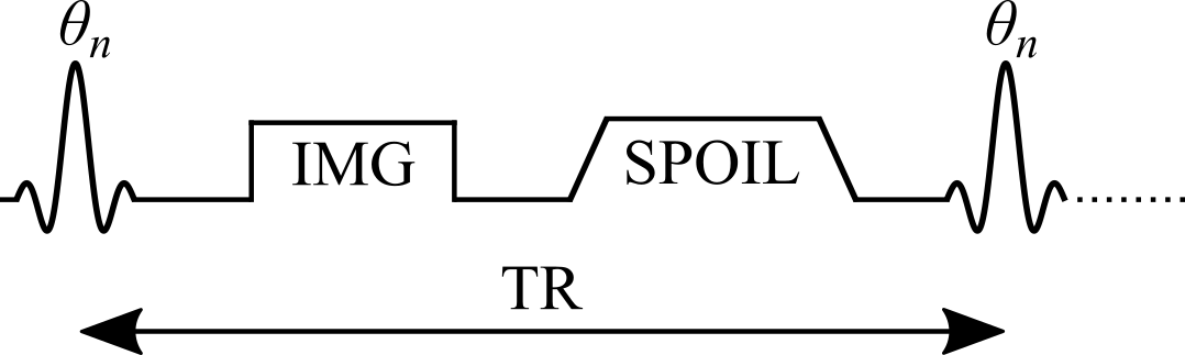
Figure 2.7:Simplified pulse sequence diagram of a variable flip angle (VFA) pulse sequence with a gradient echo readout. TR: repetition time, : excitation flip angle for the nth measurement, IMG: image acquisition (k-space readout), SPOIL: spoiler gradient.
Signal Modelling
The steady-state longitudinal magnetization of an ideal variable flip angle experiment can be analytically solved from the Bloch equations for the spoiled gradient echo pulse sequence \theta_{n}–TR}:
where Mz is the longitudinal magnetization, M0 is the magnetization at thermal equilibrium, TR is the pulse sequence repetition time (Figure 2.7), and is the excitation flip angle. The Mz curves of different T1 values for a range of and TR values are shown in Figure 2.8.
Figure 2.8:Variable flip angle technique signal curves (Eq. 2.5) for three different T1 values, approximating the main types of tissue in the brain at 3T.
From Figure 2.8, it is clearly seen that the flip angle at which the steady-state signal is maximized is dependent on the T1 and TR values. This flip angle is a well known quantity, called the Ernst angle Ernst & Anderson, 1966, which can be solved analytically from Eq. 2.5 using properties of calculus:
The closed-form solution (Eq. 2.5) makes several assumptions which in practice may not always hold true if care is not taken. Mainly, it is assumed that the longitudinal magnetization has reached a steady state after a large number of TRs, and that the transverse magnetization is perfectly spoiled at the end of each TR. Bloch simulations – a numerical approach at solving the Bloch equations for a set of spins at each time point – provide a more realistic estimate of the signal if the number of repetition times is small (i.e. a steady-state is not achieved). As can be seen from Figure 2.9, the number of repetitions required to reach a steady state not only depends on T1, but also on the flip angle; flip angles near the Ernst angle need more TRs to reach a steady state. Preparation pulses or an outward-in k-space acquisition pattern are typically sufficient to reach a steady state by the time that the center of k-space is acquired, which is where most of the image contrast resides.
Figure 2.9:Signal curves simulated using Bloch simulations (orange) for a number of repetitions ranging from 1 to 150, plotted against the ideal case (Eq. 2.5 – blue). Simulation details: TR = 25 ms, T1 = 900 ms, 100 spins. Ideal spoiling was used for this set of Bloch simulations (transverse magnetization was set to 0 at the end of each TR).
Sufficient spoiling is likely the most challenging parameter to control for in a VFA experiment. A combination of both gradient spoiling and RF phase spoiling Bernstein et al., 2004Zur et al., 1991 are typically recommended (Figure 2.10). It has also been shown that the use of very strong gradients, introduces diffusion effects (not considered in Figure 2.10), further improving the spoiling efficacy in the VFA pulse sequence Yarnykh, 2010.
Figure 2.10:Signal curves estimated using Bloch simulations for three categories of signal spoiling: (1) ideal spoiling (blue), gradient & RF Spoiling (orange), and no spoiling (green). Simulations details: TR = 25 ms, T1 = 900 ms, T2 = 100 ms, TE = 5 ms, 100 spins. For the ideal spoiling case, the transverse magnetization is set to zero at the end of each TR. For the gradient & RF spoiling case, each spin is rotated by different increments of phase (2𝜋 / # of spins) to simulate complete decoherence from gradient spoiling, and the RF phase of the excitation pulse is Bernstein et al., 2004 with = 117° Zur et al., 1991 after each TR.
Click here to view the qMRLab (MATLAB/Octave) code that generated Figure 2.8.
% Verbosity level 0 overrides the disp function and supresses warnings.
% Once executed, they cannot be restored in this session
% (kernel needs to be restarted or a new notebook opened.)
VERBOSITY_LEVEL = 0;

if VERBOSITY_LEVEL==0
    % This hack was used to supress outputs from external tools
    % in the Jupyter Book.
    function disp(x)
    end
    warning('off','all')
end

try
    cd qMRLab
catch
    try
        cd ../../../qMRLab
    catch
        cd ../qMRLab
    end
end

startup
clear all

%% Setup parameters
% All times are in milliseconds
% All flip angles are in degrees

TR_range = 5:5:200;

params.EXC_FA = 1:90;

%% Calculate signals
%
% To see all the options available, run `help vfa_t1.analytical_solution`

for ii = 1:length(TR_range)
    params.TR = TR_range(ii);

    % White matter
    params.T1 = 900; % in milliseconds

    signal_WM(ii,:) = vfa_t1.analytical_solution(params);

    % Grey matter
    params.T1 = 1500;  % in milliseconds
    signal_GM(ii,:) = vfa_t1.analytical_solution(params);

    % CSF
    params.T1 = 4000;  % in milliseconds
    signal_CSF(ii,:) = vfa_t1.analytical_solution(params);
end
Click here to view the qMRLab (MATLAB/Octave) code that generated Figure 2.9.
% Verbosity level 0 overrides the disp function and supresses warnings.
% Once executed, they cannot be restored in this session
% (kernel needs to be restarted or a new notebook opened.)
VERBOSITY_LEVEL = 0;

if VERBOSITY_LEVEL==0
    % This hack was used to supress outputs from external tools
    % in the Jupyter Book.
    function disp(x)
    end
    warning('off','all')
end

try
    cd qMRLab
catch
    try
        cd ../../../qMRLab
    catch
        cd ../qMRLab
    end
end

startup
clear all

%% Setup parameters
% All times are in milliseconds
% All flip angles are in degrees

% White matter
params.T1 = 900; % in milliseconds
params.T2 = 10000;
params.TR = 25;
params.TE = 5;
params.EXC_FA = 1:90;
Nex_range = 1:1:150;

%% Calculate signals
%
% To see all the options available, run `help vfa_t1.analytical_solution`

for ii = 1:length(Nex_range)
    params.Nex = Nex_range(ii);

    signal_analytical(ii,:) = vfa_t1.analytical_solution(params);

    [~, complex_signal] = vfa_t1.bloch_sim(params);
    signal_blochsim(ii,:) = abs(complex(complex_signal));
end
Click here to view the qMRLab (MATLAB/Octave) code that generated Figure 2.10.
% Verbosity level 0 overrides the disp function and supresses warnings.
% Once executed, they cannot be restored in this session
% (kernel needs to be restarted or a new notebook opened.)
VERBOSITY_LEVEL = 0;

if VERBOSITY_LEVEL==0
    % This hack was used to supress outputs from external tools
    % in the Jupyter Book.
    function disp(x)
    end
    warning('off','all')
end

try
    cd qMRLab
catch
    try
        cd ../../../qMRLab
    catch
        cd ../qMRLab
    end
end

startup
clear all

%% Setup parameters
% All times are in milliseconds
% All flip angles are in degrees

% White matter
params.T1 = 900; % in milliseconds
params.T2 = 100;
params.TR = 25;
params.TE = 5;
params.EXC_FA = 1:90;
Nex_range = [1:9, 10:10:100];

%% Calculate signals
%
% To see all the options available, run `help vfa_t1.analytical_solution`

for ii = 1:length(Nex_range)
    params.Nex = Nex_range(ii);

    params.crushFlag = 1;

    [~, complex_signal] = vfa_t1.bloch_sim(params);
    signal_ideal_spoil(ii,:) = abs(complex_signal);


    params.inc = 117;
    params.partialDephasing = 1;
    params.partialDephasingFlag = 1;
    params.crushFlag = 0;

    [~, complex_signal] = vfa_t1.bloch_sim(params);
    signal_optimal_crush_and_rf_spoil(ii,:) = abs(complex_signal);

    params.inc = 0;
    params.partialDephasing = 0;

    [~, complex_signal] = vfa_t1.bloch_sim(params);
    signal_no_gradient_and_rf_spoil(ii,:) = abs(complex_signal);
end
Data Fitting
At first glance, one could be tempted to fit VFA data using a non-linear least squares fitting algorithm such as Levenberg-Marquardt with Eq. 2.5, which typically only has two free fitting variables (T1 and M0). Although this is a valid way of estimating T1 from VFA data, it is rarely done in practice because a simple refactoring of Eq. 2.5 allows T1 values to be estimated with a linear least square fitting algorithm, which substantially reduces the processing time. Without any approximations, Eq. 2.5 can be rearranged into the form Gupta, 1977:
As the third term does not change between measurements (it is constant for each ), it can be grouped into the constant for a simpler representation:
With this rearranged form of Eq. 2.5, T1 can be simply estimated from the slope of a linear regression calculated from and values:
If data were acquired using only two flip angles – a very common VFA acquisition protocol – then the slope can be calculated using the elementary slope equation. Figure 2.11 displays both Equations Eq. 2.5 and Eq. 2.8 plotted for a noisy dataset.
Figure 2.11:Mean and standard deviation of the VFA signal plotted using the nonlinear form (Eq. 2.5 – blue) and linear form (Eq. 2.8 – red). Monte Carlo simulation details: SNR = 25, N = 1000. VFA simulation details: TR = 25 ms, T1 = 900 ms.
There are two important imaging protocol design considerations that should be taken into account when planning to use VFA: (1) how many and which flip angles to use to acquire VFA data, and (2) correcting inaccurate flip angles due to transmit RF field inhomogeneity. Most VFA experiments use the minimum number of required flip angles (two) to minimize acquisition time. For this case, it has been shown that the flip angle choice resulting in the best precision for VFA T1 estimates for a sample with a single T1 value (i.e. single tissue) are the two flip angles that result in 71% of the maximum possible steady-state signal (i.e. at the Ernst angle) Deoni et al., 2003Schabel & Morrell, 2008.
Time allowing, additional flip angles are often acquired at higher values and in between the two above, because greater signal differences between tissue T1 values are present there (e.g. Figure 2.8). Also, for more than two flip angles, Equations Eq. 2.5 and Eq. 2.8 do not have the same noise weighting for each fitting point, which may bias linear least-square T1 estimates at lower SNRs. Thus, it has been recommended that low SNR data should be fitted with either Eq. 2.5 using non-linear least-squares (slower fitting) or with a weighted linear least-square form of Eq. 2.8 Chang et al., 2008.
Accurate knowledge of the flip angle values is very important to produce accurate T1 maps. Because of how the RF field interacts with matter Sled & Pike, 1998, the excitation RF field (B1+, or B1 for short) of a loaded RF coil results in spatial variations in intensity/amplitude, unless RF shimming is available to counteract this effect (not common at clinical field strengths). For quantitative measurements like VFA which are sensitive to this parameter, the flip angle can be corrected (voxelwise) relative to the nominal value by multiplying it with a scaling factor (B1) from a B1 map that is acquired during the same session:
B1 in this context is normalized, meaning that it is unitless and has a value of 1 in voxels where the RF field has the expected amplitude (i.e. where the nominal flip angle is the actual flip angle). Figure 2.11 displays fitted VFA T1 values from a Monte Carlo dataset simulated using biased flip angle values, and fitted without/with B1 correction.
Figure 2.11:Mean and standard deviations of fitted VFA T1 values for a set of Monte Carlo simulations (SNR = 100, N = 1000), simulated using a wide range of biased flip angles and fitted without (blue) or with (red) B1 correction. Simulation parameters: TR = 25 ms, T1 = 900 ms, = 6° and 32° (optimized values for this TR/T1 combination). Notice how even after B1 correction, fitted T1 values at B1 values far from the nominal case (B1 = 1) exhibit larger variance, as the actual flip angles of the simulated signal deviate from the optimal values for this TR/T1 (Deoni et al. 2003).
Figure 2.12 displays an example VFA dataset and a B1 map in a healthy brain, along with the T1 map estimated using a linear fit (Equations Eq. 2.8 and Eq. 2.9).
Figure 2.12:Example variable flip angle dataset and B1 map of a healthy adult brain (left). The relevant VFA protocol parameters used were: TR = 15 ms, = 3° and 20°. The T1 map (right) was fitted using a linear regression (Equations Eq. 2.8 and Eq. 2.9).
Click here to view the qMRLab (MATLAB/Octave) code that generated Figure 2.11.
% Verbosity level 0 overrides the disp function and supresses warnings.
% Once executed, they cannot be restored in this session
% (kernel needs to be restarted or a new notebook opened.)
VERBOSITY_LEVEL = 0;

if VERBOSITY_LEVEL==0
    % This hack was used to supress outputs from external tools
    % in the Jupyter Book.
    function disp(x)
    end
    warning('off','all')
end

try
    cd qMRLab
catch
    try
        cd ../../../qMRLab
    catch
        cd ../qMRLab
    end
end

startup
clear all

%% Setup parameters
% All times are in milliseconds
% All flip angles are in degrees

params.EXC_FA = [1:4,5:5:90];

%% Calculate signals
%
% To see all the options available, run `help vfa_t1.analytical_solution`

params.TR = 0.025;
params.EXC_FA = [2:9,10:5:90];

% White matter
x.M0 = 1;
x.T1 = 0.900; % in milliseconds

Model = vfa_t1;

Opt.SNR = 25;
Opt.TR = params.TR;
Opt.T1 = x.T1;

clear Model.Prot.VFAData.Mat(:,1)
Model.Prot.VFAData.Mat = zeros(length(params.EXC_FA),2);
Model.Prot.VFAData.Mat(:,1) = params.EXC_FA';
Model.Prot.VFAData.Mat(:,2) = Opt.TR;

for jj = 1:1000
    [FitResult{jj}, noisyData{jj}] = Model.Sim_Single_Voxel_Curve(x,Opt,0);
    fittedT1(jj) = FitResult{jj}.T1;
    noisyData_array(jj,:) = noisyData{jj}.VFAData;
    noisyData_array_div_sin(jj,:) = noisyData_array(jj,:) ./ sind(Model.Prot.VFAData.Mat(:,1))';
    noisyData_array_div_tan(jj,:) = noisyData_array(jj,:) ./ tand(Model.Prot.VFAData.Mat(:,1))';
end

for kk=1:length(params.EXC_FA)
    data_mean(kk) = mean(noisyData_array(:,kk));
    data_std(kk) = std(noisyData_array(:,kk));

    data_mean_div_sin(kk) = mean(noisyData_array_div_sin(:,kk));
    data_std_div_sin(kk) = std(noisyData_array_div_sin(:,kk));

    data_mean_div_tan(kk) = mean(noisyData_array_div_tan(:,kk));
    data_std_div_tan(kk) = std(noisyData_array_div_tan(:,kk));
end


%% Setup parameters
% All times are in milliseconds
% All flip angles are in degrees

params_highres.EXC_FA = [2:1:90];

%% Calculate signals
%
% To see all the options available, run `help vfa_t1.analytical_solution`

params_highres.TR = params.TR * 1000; % in milliseconds

% White matter
params_highres.T1 = x.T1*1000; % in milliseconds

signal_WM = vfa_t1.analytical_solution(params_highres);
signal_WM_div_sin = signal_WM ./ sind(params_highres.EXC_FA);
signal_WM_div_tan = signal_WM ./ tand(params_highres.EXC_FA);
Click here to view the qMRLab (MATLAB/Octave) code that generated Figure 2.11.
% Verbosity level 0 overrides the disp function and supresses warnings.
% Once executed, they cannot be restored in this session
% (kernel needs to be restarted or a new notebook opened.)
VERBOSITY_LEVEL = 0;

if VERBOSITY_LEVEL==0
    % This hack was used to supress outputs from external tools
    % in the Jupyter Book.
    function disp(x)
    end
    warning('off','all')
end

try
    cd qMRLab
catch
    try
        cd ../../../qMRLab
    catch
        cd ../qMRLab
    end
end

startup
clear all

%% Setup parameters
% All times are in seconds
% All flip angles are in degrees

params.TR = 0.025; % in seconds

% White matter
params.T1 = 0.900; % in seconds

% Calculate optimal flip angles for a two flip angle VFA experiment (for this T1 and TR)
% The will be the nominal flip angles (the flip angles assumed by the "user", before a
% "realistic"B1 bias is applied)

nominal_EXC_FA = vfa_t1.find_two_optimal_flip_angles(params); % in degrees
disp('Nominal flip angles:')
disp(nominal_EXC_FA)

% Range of B1 values biasing the excitation flip angle away from their nominal values
B1Range = 0.1:0.1:2;

x.M0 = 1;
x.T1 = params.T1; % in seconds

Model = vfa_t1;

Opt.SNR = 100;
Opt.TR = params.TR;
Opt.T1 = x.T1;

% Monte Carlo signal simulations
for ii = 1:1000
    for jj = 1:length(B1Range)
        B1 = B1Range(jj);
        actual_EXC_FA = B1 * nominal_EXC_FA;

        params.EXC_FA = actual_EXC_FA;

        clear Model.Prot.VFAData.Mat(:,1)
        Model.Prot.VFAData.Mat = zeros(length(params.EXC_FA),2);
        Model.Prot.VFAData.Mat(:,1) = params.EXC_FA';
        Model.Prot.VFAData.Mat(:,2) = Opt.TR;

        [FitResult{ii,jj}, noisyData{ii,jj}] = Model.Sim_Single_Voxel_Curve(x,Opt,0);
        noisyData_array(ii,jj,:) = noisyData{ii,jj}.VFAData;
    end
end
%
Model = vfa_t1;

FlipAngle = nominal_EXC_FA';
TR = params.TR .* ones(size(FlipAngle));

Model.Prot.VFAData.Mat = [FlipAngle TR];

data.VFAData(:,:,1,1) = noisyData_array(:,:,1);
data.VFAData(:,:,1,2) = noisyData_array(:,:,2);
data.Mask = repmat(ones(size(B1Range)),[size(noisyData_array,1),1]);

data.B1map = repmat(ones(size(B1Range)),[size(noisyData_array,1),1]);
FitResults_noB1Correction = FitData(data,Model,0);

data.B1map = repmat(B1Range,[size(noisyData_array,1),1]);
FitResults_withB1Correction = FitData(data,Model,0);

%%
%

mean_T1_noB1Correction = mean(FitResults_noB1Correction.T1);
mean_T1_withB1Correction = mean(FitResults_withB1Correction.T1);
std_T1_noB1Correction = std(FitResults_noB1Correction.T1);
std_T1_withB1Correction = std(FitResults_withB1Correction.T1);
Click here to view the qMRLab (MATLAB/Octave) code that generated Figure 2.12.
% Verbosity level 0 overrides the disp function and supresses warnings.
% Once executed, they cannot be restored in this session
% (kernel needs to be restarted or a new notebook opened.)
VERBOSITY_LEVEL = 0;

if VERBOSITY_LEVEL==0
    % This hack was used to supress outputs from external tools
    % in the Jupyter Book.
    function disp(x)
    end
    warning('off','all')
end

try
    cd qMRLab
catch
    try
        cd ../../../qMRLab
    catch
        cd ../qMRLab
    end
end

startup
clear all

%% MATLAB/OCTAVE CODE

% Load data into environment, and rotate mask to be aligned with IR data
load('data/vfa_dataset/VFAData.mat');
load('data/vfa_dataset/B1map.mat');
load('data/vfa_dataset/Mask.mat');

% Format qMRLab vfa_t1 model parameters, and load them into the Model object
Model = vfa_t1;
FlipAngle = [    3;     20];
TR        = [0.015; 0.0150];

Model.Prot.VFAData.Mat = [FlipAngle, TR];

% Format data structure so that they may be fit by the model
data = struct();
data.VFAData= double(VFAData);
data.B1map= double(B1map);
data.Mask= double(Mask);

FitResults = FitData(data,Model,0); % The '0' flag is so that no wait bar is shown.

T1_map = imrotate(FitResults.T1.*Mask,-90);
T1_map(T1_map>5)=0;
T1_map = T1_map*1000; % Convert to ms

xAxis = [0:size(T1_map,2)-1];
yAxis = [0:size(T1_map,1)-1];

% Raw MRI data at different TI values
FA_03 = imrotate(squeeze(VFAData(:,:,:,1).*Mask),-90);
FA_20 = imrotate(squeeze(VFAData(:,:,:,2).*Mask),-90);
B1map = imrotate(squeeze(B1map.*Mask),-90);
Benefits and Pitfalls
It has been well reported in recent years that the accuracy of VFA T1 estimates is very sensitive to pulse sequence implementations Baudrexel et al., 2017Lutti & Weiskopf, 2013Stikov et al., 2015, and as such is less robust than the gold standard inversion recovery technique. In particular, the signal bias resulting from insufficient spoiling can result in inaccurate T1 estimates of up to 30% relative to inversion recovery estimated values Stikov et al., 2015. VFA T1 map accuracy and precision is also strongly dependent on the quality of the measured B1 map Lee et al., 2017, which can vary substantially between implementations Boudreau et al., 2017. Modern rapid B1 mapping pulse sequences are not as widely available as VFA, resulting in some groups attempting alternative ways of removing the bias from the T1 maps like generating an artificial B1 map through the use of image processing techniques Liberman et al., 2013 or omitting B1 correction altogether Yuan et al., 2012. The latter is not recommended, because most MRI scanners have default pulse sequences that, with careful protocol settings, can provide B1 maps of sufficient quality very rapidly Boudreau et al., 2017Samson et al., 2006Wang et al., 2005.
Despite some drawbacks, VFA is still one of the most widely used T1 mapping methods in research. Its rapid acquisition time, rapid image processing time, and widespread availability makes it a great candidate for use in other quantitative imaging acquisition protocols like quantitative magnetization transfer imaging Cercignani et al., 2005Yarnykh, 2002 and dynamic contrast enhanced imaging Li et al., 2018Sung et al., 2013.
4MP2RAGE
Dictionary-based MRI techniques capable of generating T1 maps are increasing in popularity, due to their growing availability on clinical scanners, rapid scan times, and fast post-processing computation time, thus making quantitative T1 mapping accessible for clinical applications. Generally speaking, dictionary-based quantitative MRI techniques use numerical dictionaries—databases of pre-calculated signal values simulated for a wide range of tissue and protocol combinations—during the image reconstruction or post-processing stages. Popular examples of dictionary-based techniques that have been applied to T1 mapping are MR Fingerprinting (MRF) Ma et al., 2013, certain flavours of compressed sensing (CS) Doneva et al., 2010Li et al., 2012, and Magnetization Prepared 2 Rapid Acquisition Gradient Echoes (MP2RAGE) Marques et al., 2010. Dictionary-based techniques can usually be classified into one of two categories: techniques that use information redundancy from parametric data to assist in accelerated imaging (e.g. CS, MRF), or those that use dictionaries to estimate quantitative maps using the MR images after reconstruction. Because MP2RAGE is a technique implemented primarily for T1 mapping, and it is becoming increasingly available as a standard pulse sequence on many MRI systems, the remainder of this section will focus solely on this technique. However, many concepts discussed are shared by other dictionary-based techniques.
MP2RAGE is an extension of the conventional MPRAGE pulse sequence widely used in clinical studies Haase et al., 1989Mugler & Brookeman, 1990. A simplified version of the MP2RAGE pulse sequence is shown in Figure 2.13. MP2RAGE can be seen as a hybrid between the inversion recovery and VFA pulse sequences: a 180° inversion pulse is used to prepare the magnetization for T1 sensitivity at the beginning of each TRMP2RAGE, and then two images are acquired at different inversion times using gradient recalled echo (GRE) imaging blocks with low flip angles and short repetition times (TR). During a given GRE imaging block, each excitation pulse is followed by a constant in-plane (“y”) phase encode weighting (varied for each TRMP2RAGE), but with different 3D (“z”) phase encoding gradients (varied at each TR). The center of k-space for the 3D phase encoding direction is acquired at the TI for each GRE imaging block. The main motivation for developing the MP2RAGE pulse sequence was to provide a metric similar to MPRAGE, but with self-bias correction of the static (B0) and receive (B1-) magnetic fields, and a first order correction of the transmit magnetic field (B1+). However, because two images at different TIs are acquired (unlike MPRAGE, which only acquires data at a single TI), information about the T1 values can also be inferred, thus making it possible to generate quantitative T1 maps using this data.
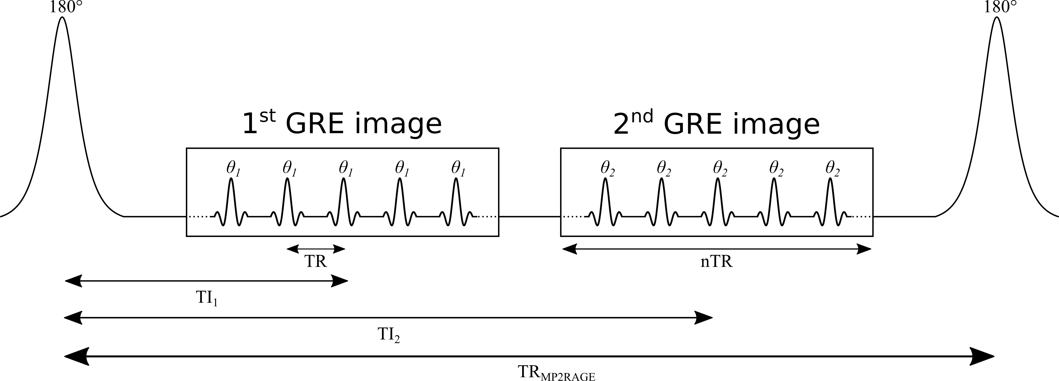
Figure 2.13:Simplified diagram of an MP2RAGE pulse sequence. TR: repetition time between successive gradient echo readouts, TRMP2RAGE: repetition time between successive adiabatic 180° inversion pulses, TI1 and TI2: inversion times, and : excitation flip angles. The imaging readout events occur within each TR using a constant in-plane phase encode (“y”) gradient set for each TRMP2RAGE, but varying 3D phase encode (“z”) gradients between each successive TR.
Signal Modelling
Prior to considering the full signal equations, we will first introduce the equation for the MP2RAGE parameter (SMP2RAGE) that is calculated in addition to the T1 map. For complex data (magnitude and phase, or real and imaginary), the MP2RAGE signal (SMP2RAGE) is calculated from the images acquired at two TIs (SGRE,TI1 and SGRE,TI2) using the following expression Marques et al., 2010:
This value is bounded between [-0.5, 0.5], and helps reduce some B0 inhomogeneity effects using the phase data. For real data, or magnitude data with polarity restoration, this metric is instead calculated as:
Because MP2RAGE is a hybrid of pulse sequences used for inversion recovery and VFA, the resulting signal equations are more complex. Typically, a steady state is not achieved during the short train of GRE imaging blocks, so the signal at the center of k-space for each readout (which defines the contrast weighting) will depend on the number of phase-encoding steps. For simplicity, the equations presented here assume that the 3D phase-encoding dimension is fully sampled (no partial Fourier or parallel imaging acceleration). For this case (see appendix of Marques et al., 2010 for derivation details), the signal equations are:
where B1- is the receive field sensitivity, “eff” is the adiabatic inversion pulse efficiency, ER=exp(-TR/T1), EA=exp(-TA/T1), EB=exp(-TB/T1), EC=exp(-TC/T1). The variables TA, TB, and TC are the three different delay times (TA: time between inversion pulse and beginning of the GRE1 block, TB: time between the end of GRE1 and beginning of GRE2, TC: time between the end of GRE2 and the end of the TR). If no k-space acceleration is used (e.g. no partial Fourier or parallel imaging acceleration), then these values are TA = TI1 - (n/2)TR, TB = TI2 - (TI1 + nTR), and TC = TRMP2RAGE - (TI1 + (n/2)TR), where n is the number of voxels acquired in the 3D phase encode direction varied within each GRE block. The value mz,ss is the steady-state longitudinal magnetization prior to the inversion pulse, and is given by:
From Equations 2.13, 2.14, 2.15, and 2.16, it is evident that the MP2RAGE parameter SMP2RAGE (Equations 2.11, 2.12) cancels out the effects of receive field sensitivity, T2*, and M0. The signal sensitivity related to the transmit field (B1+), hidden in Equations 2.13, 2.14, 2.15, and 2.16 within the flip angle values and , can also be reduced by careful pulse sequence protocol design Marques et al., 2010, but not entirely eliminated Marques & Gruetter, 2013.
Data Fitting
Dictionary-based techniques such as MP2RAGE do not typically use conventional minimization algorithms (e.g. Levenberg-Marquardt to fit signal equations to observed data. Instead, the MP2RAGE technique uses pre-calculated signal values for a wide range of parameter values (e.g. T1), and then interpolation is done within this dictionary of values to estimate the T1 value that matches the observed signal. This approach results in rapid post-processing times because the dictionaries can be simulated/generated prior to scanning and interpolating between these values is much faster than most fitting algorithms. This means that the quantitative image can be produced and displayed directly on the MRI scanner console rather than needing to be fitted offline.
Figure 2.14:T1 lookup table as a function of T1 and SMP2RAGE value. Inversion times used to acquire this magnitude image dataset were 800 ms and 2700 ms, the flip angles were 4° and 5° (respectively), TRMP2RAGE = 6000 ms, and TR = 6.7 ms. The code that was used were shared open sourced by the authors of the original MP2RAGE paper Marques, 2017.
To produce T1 maps with good accuracy and precision using dictionary-based interpolation methods, it is important that the signal curves are unique for each parameter value. MP2RAGE can produce good T1 maps by using a dictionary with only dimensions (T1, SMP2RAGE), since SMP2RAGE is unique for each T1 value for a given protocol Marques et al., 2010. However, as was noted above, SMP2RAGE is also sensitive to B1 because of and in Equations 2.13, 2.14, 2.15, and 2.16. The B1-sensitivity can be reduced substantially with careful MP2RAGE protocol optimization Marques et al., 2010, and further improved by including B1 as one of the dictionary dimensions [T1, B1, SMP2RAGE] (Figure 2.14). This requires an additional acquisition of a B1 map Marques & Gruetter, 2013, which lengthens the scan time.
Figure 2.15:Example MP2RAGE dataset of a healthy adult brain at 7T and T1 map. Inversion times used to acquire this magnitude image dataset were 800 ms and 2700 ms, the flip angles were 4° and 5° (respectively), TRMP2RAGE = 6000 ms, and TR = 6.7 ms. The dataset and code that was used were shared open sourced by the authors of the original MP2RAGE paper Marques, 2017.
The MP2RAGE pulse sequence is increasingly being distributed by MRI vendors, thus typically a data fitting package is also available to reconstruct the T1 maps online. Alternatively, several open source packages to create T1 maps from MP2RAGE data are available online Marques, 2017Hollander, 2017, and for new users these are recommended—as opposed to programming one from scratch—as there are many potential pitfalls (e.g. adjusting the equations to handle partial Fourier or parallel imaging acceleration).
Benefits and Pitfalls
This widespread availability and its turnkey acquisition/fitting procedures are a main contributing factor to the growing interest for including quantitative T1 maps in clinical and neuroscience studies. T1 values measured using MP2RAGE showed high levels of reproducibility for the brain in an inter- and intra-site study at eight sites (same MRI hardware/software and at 7 T) of two subjects Voelker et al., 2016. Not only does MP2RAGE have one of the fastest acquisition and post-processing times among quantitative T1 mapping techniques, but it can accomplish this while acquiring very high resolution T1 maps (1 mm isotropic at 3T and submillimeter at 7T, both in under 10 min Fujimoto et al., 2014), opening the doors to cortical studies which greatly benefit from the smaller voxel size Waehnert et al., 2014Beck et al., 2018Haast et al., 2018.
Despite these benefits, MP2RAGE and similar dictionary-based techniques have certain limitations that are important to consider before deciding to incorporate them in a study. Good reproducibility of the quantitative T1 map is dependent on using one pre-calculated dictionary. If two different dictionaries are used (e.g. cross-site with different MRI vendors), the differences in the dictionary interpolations will likely result in minor differences in T1 estimates for the same data. Also, although the B1-sensitivity of the MP2RAGE T1 maps can be reduced with proper protocol optimization, it can be substantial enough that further correction using a measured B1 map should be done Marques & Gruetter, 2013Haast et al., 2018. However B1 mapping brings an additional potential source of error, so carefully selecting a B1 mapping technique and accompanying post-processing method (e.g. filtering) should be done before integrating it in a T1 mapping protocol Boudreau et al., 2017. Lastly, the MP2RAGE equations (and thus, dictionaries) assume monoexponential longitudinal relaxation, and this has been shown to result in suboptimal estimates of the long T1 component for a biexponential relaxation model Rioux et al., 2016, an effect that becomes more important at higher fields.
5Exercises
- Ernst, R. R., & Anderson, W. A. (1966). Application of Fourier Transform Spectroscopy to Magnetic Resonance. Review of Scientific Instruments, 37(1), 93–102. 10.1063/1.1719961
- Cercignani, M., Symms, M. R., Schmierer, K., Boulby, P. A., Tozer, D. J., Ron, M., Tofts, P. S., & Barker, G. J. (2005). Three-dimensional quantitative magnetisation transfer imaging of the human brain. NeuroImage, 27(2), 436–441. 10.1016/j.neuroimage.2005.04.031
- Yarnykh, V. L. (2002). Pulsed Z-spectroscopic imaging of cross-relaxation parameters in tissues for human MRI: Theory and clinical applications. Magnetic Resonance in Medicine, 47(5), 929–939. 10.1002/mrm.10120
- Li, Z. F., Zhao, W., Qi, T. F., Gao, C., Gu, Q., Zhao, J. S., & Koh, T. S. (2018). A simple B1correction method for dynamic contrast-enhanced MRI. Physics in Medicine and Biology, 63(16), 16NT01. 10.1088/1361-6560/aad519
- Sung, K., Daniel, B. L., & Hargreaves, B. A. (2013). Transmit field inhomogeneity and T1 estimation errors in breast DCE-MRI at 3 tesla. Journal of Magnetic Resonance Imaging, 38(2), 454–459. 10.1002/jmri.23996
- Stikov, N., Boudreau, M., Levesque, I. R., Tardif, C. L., Barral, J. K., & Pike, G. B. (2015). On the accuracy of T1 mapping: Searching for common ground. Magnetic Resonance in Medicine, 73(2), 514–522. 10.1002/mrm.25135
- Steen, R. G., Gronemeyer, S. A., Kingsley, P. B., Reddick, W. E., Langston, J. S., & Taylor, J. S. (1994). Precise and accurate measurement of proton T1 in human brain in vivo: validation and preliminary clinical application. Journal of Magnetic Resonance Imaging, 4(5), 681–691. 10.1002/jmri.1880040511
- Christensen, K. A., Grant, D. M., Schulman, E. M., & Walling, C. (1974). Optimal determination of relaxation times of Fourier transform nuclear magnetic resonance. Determination of spin-lattice relaxation times in chemically polarized species. The Journal of Physical Chemistry, 78(19), 1971–1977. 10.1021/j100612a022
- Fram, E. K., Herfkens, R. J., Johnson, G. A., Glover, G. H., Karis, J. P., Shimakawa, A., Perkins, T. G., & Pelc, N. J. (1987). Rapid calculation of T1 using variable flip angle gradient refocused imaging. Magnetic Resonance Imaging, 5(3), 201–208. 10.1016/0730-725x(87)90021-x
- Gupta, R. K. (1977). A new look at the method of variable nutation angle for the measurement of spin-lattice relaxation times using fourier transform NMR. Journal of Magnetic Resonance (1969), 25(1), 231–235. 10.1016/0022-2364(77)90138-x
- Sled, J. G., & Pike, G. B. (1998). Standing-wave and RF penetration artifacts caused by elliptic geometry: an electrodynamic analysis of MRI. IEEE Transactions on Medical Imaging, 17(4), 653–662. 10.1109/42.730409
- Boudreau, M., Tardif, C. L., Stikov, N., Sled, J. G., Lee, W., & Pike, G. B. (2017). B1 mapping for bias-correction in quantitative T1 imaging of the brain at 3T using standard pulse sequences. Journal of Magnetic Resonance Imaging, 46(6), 1673–1682. 10.1002/jmri.25692
- Marques, J. P., Kober, T., Krueger, G., van der Zwaag, W., Van de Moortele, P.-F., & Gruetter, R. (2010). MP2RAGE, a self bias-field corrected sequence for improved segmentation and T1-mapping at high field. Neuroimage, 49(2), 1271–1281.
- Hahn, E. L. (1949). An accurate nuclear magnetic resonance method for measuring spin-lattice relaxation times. Physical Review, 76(1), 145. 10.1103/PhysRev.76.145
- Drain, L. (1949). A direct method of measuring nuclear spin-lattice relaxation times. Proceedings of the Physical Society. Section A, 62(5), 301. 10.1088/0370-1298/62/5/306