import nibabel as nib
import os
import numpy as np
import matplotlib.pyplot as plt
from contextlib import contextmanager
import sys, os
from pathlib import Path
@contextmanager
def suppress_stdout():
with open(os.devnull, "w") as devnull:
old_stdout = sys.stdout
sys.stdout = devnull
try:
yield
finally:
sys.stdout = old_stdout
import os
from pathlib import Path
def find_myst_yml_directories(start_dir=None):
"""
Recursively search for directories containing myst.yml file.
Args:
start_dir (str or Path): Starting directory (defaults to current directory)
Returns:
list: List of full paths to directories containing myst.yml
"""
if start_dir is None:
start_dir = Path.cwd()
else:
start_dir = Path(start_dir)
myst_dirs = []
def _search_directory(current_dir):
# Check if myst.yml exists in current directory
myst_file = current_dir / "myst.yml"
if myst_file.exists():
myst_dirs.append(str(current_dir.resolve()))
# Don't search subdirectories if we found myst.yml here
return
# Recursively search all subdirectories
for item in current_dir.iterdir():
if item.is_dir():
try:
_search_directory(item)
except (PermissionError, OSError):
# Skip directories we can't access
continue
_search_directory(start_dir)
return myst_dirs
def find_myst_yml_directories_upwards(start_dir=None):
"""
Search for myst.yml in current directory, if not found go to parent and repeat.
Args:
start_dir (str or Path): Starting directory (defaults to current directory)
Returns:
str or None: Full path of directory containing myst.yml, or None if not found
"""
if start_dir is None:
current_dir = Path.cwd()
else:
current_dir = Path(start_dir)
# Keep going up until we reach the filesystem root
while current_dir != current_dir.parent: # Stop at root
myst_file = current_dir / "myst.yml"
if myst_file.exists():
return str(current_dir.resolve())
# Move to parent directory
current_dir = current_dir.parent
return None
with suppress_stdout():
repo_path = Path(find_myst_yml_directories_upwards())
print(repo_path)
data_req_path = repo_path / "binder" / "data_requirement.json"
data_path = repo_path / "data"
dataset_path = data_path / "qmrlab-mooc"
data_dir = dataset_path / "07-Applications" / "07-Applications"
# SPGR function
def spgr(constant, T1, T2, TR, TE, FA):
return (constant * ((1 - np.exp(-TR / T1)) / (1 - np.cos(FA) * np.exp(-TR / T1)))* np.sin(FA))*np.exp(-TE/T2)
def ir(constant, T1, T2, TR, TI, TE, FA):
return constant * ((1- np.cos(np.pi) * np.exp(-TR / T1)- (1 - np.cos(np.pi))* np.exp(-TI / T1))/ (1- np.cos(np.pi)* np.cos(FA)* np.exp(-TR / T1)))*np.sin(FA)*np.exp(-TE/T2)
t1map = nib.load(data_dir / "FLAIR - T1 map.nii.gz").get_fdata()
# Simulate a T2 map by dividing the T1 map by 10
t2map = t1map / 10
# Get all the (x, y) ints in a grid that fall within a circle int(5) diameter for a center at (112,163)
#x, y = np.mgrid[:t1map.shape[0], :t1map.shape[1]]
#mask = (x - 115)**2 + (y - 158)**2 < 2.6**2
mask = nib.load('Mask.nii.gz').get_fdata()
mask=np.squeeze(mask)
# Introduce a circular lesion at 100 and 150
t2map[mask!=0] = t2map[mask!=0]*2
t1map[mask!=0] = t1map[mask!=0]*1.1
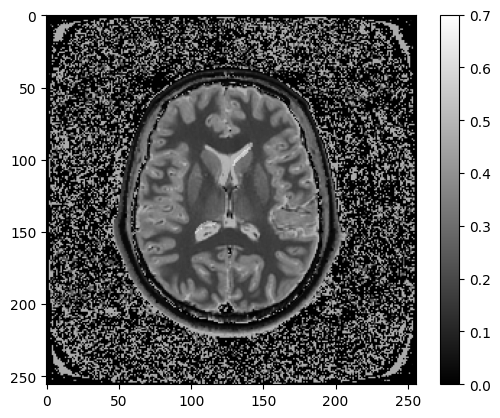
# Simulate a T2-weighted spgr image using the T1 and T2 values voxel-wise, TR = 4000 ms, TE = 100 ms, and FA = 90 degrees
TR = 5000
TE = 150
FA = 90
t2w=spgr(1, t1map, t2map, TR, TE, np.deg2rad(FA))
# Plot the T2-weighted spgr image in black and white
plt.imshow(np.rot90(t2w),cmap='grey')
plt.clim(0, 0.7)
plt.colorbar()
plt.show()
# Simulate a T1-weighted spgr image using the T1 and T2 values voxel-wise
TR = 500
TE = 15
FA = 70
t1w=spgr(1, t1map, t2map, TR, TE, np.deg2rad(FA))

# Plot the T2-weighted spgr image in black and white
plt.imshow(np.rot90(t1w),cmap='grey')
plt.clim(0, 0.6)
plt.colorbar()
plt.show()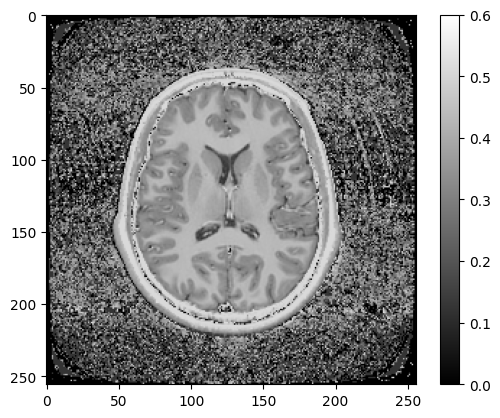
# Simulate a T2-weighted spgr image using the T1 and T2 values voxel-wise, TR = 4000 ms, TE = 100 ms, and FA = 90 degrees
TR = 5000
TI = 50
TE = 15
FA = 90

flair=ir(1, t1map, t2map, TR, TI, TE, np.deg2rad(FA))

# Plot the T2-weighted spgr image in black and white
plt.imshow(abs(np.rot90(flair)),cmap='gray')
plt.clim(0, 1.5)
plt.colorbar()
plt.show()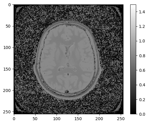
# Simulate a T2-weighted spgr image using the T1 and T2 values voxel-wise, TR = 4000 ms, TE = 100 ms, and FA = 90 degrees
TR = 5000
TI = 500
TE = 15
FA = 90

flair=ir(1, t1map, t2map, TR, TI, TE, np.deg2rad(FA))

# Plot the T2-weighted spgr image in black and white
plt.imshow(abs(np.rot90(flair)),cmap='gray')
plt.clim(0, 1)
plt.colorbar()
plt.show()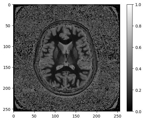
# Simulate a T2-weighted spgr image using the T1 and T2 values voxel-wise, TR = 4000 ms, TE = 100 ms, and FA = 90 degrees
TR = 5000
TI = 1000
TE = 15
FA = 90

flair=ir(1, t1map, t2map, TR, TI, TE, np.deg2rad(FA))

# Plot the T2-weighted spgr image in black and white
plt.imshow(abs(np.rot90(flair)),cmap='gray')
plt.clim(0, 1.2)
plt.colorbar()
plt.show()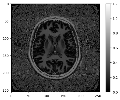
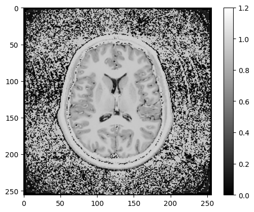
# Simulate a T2-weighted spgr image using the T1 and T2 values voxel-wise, TR = 4000 ms, TE = 100 ms, and FA = 90 degrees
TR = 5000
TI = 3000
TE = 15
FA = 90

flair=ir(1, t1map, t2map, TR, TI, TE, np.deg2rad(FA))

# Plot the T2-weighted spgr image in black and white
plt.imshow(abs(np.rot90(flair)),cmap='gray')
plt.clim(0, 1.2)
plt.colorbar()
plt.show()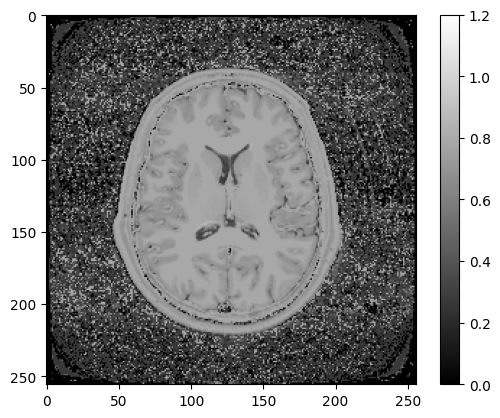
# Simulate a T2-weighted spgr image using the T1 and T2 values voxel-wise, TR = 4000 ms, TE = 100 ms, and FA = 90 degrees
TR = 10000
TI = 3000
TE = 150
FA = 90

flair=ir(1, t1map, t2map, TR, TI, TE, np.deg2rad(FA))

# Plot the T2-weighted spgr image in black and white
plt.imshow(abs(np.rot90(flair)),cmap='gray')
plt.clim(0, 0.5)
plt.colorbar()
plt.show()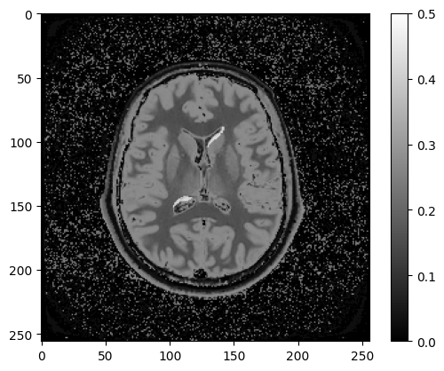
# Simulate a T2-weighted spgr image using the T1 and T2 values voxel-wise, TR = 4000 ms, TE = 100 ms, and FA = 90 degrees
TR = 5000
TI = 3000
TE = 15
FA = 20

flair=ir(1, t1map, t2map, TR, TI, TE, np.deg2rad(FA))

# Plot the T2-weighted spgr image in black and white
plt.imshow(abs(np.rot90(flair)),cmap='gray')
plt.clim(0, 0.4)
plt.colorbar()
plt.show()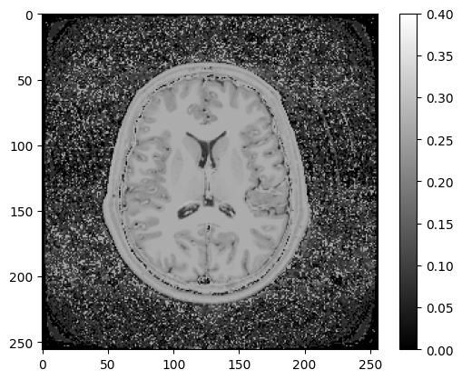
# Simulate a T2-weighted spgr image using the T1 and T2 values voxel-wise, TR = 4000 ms, TE = 100 ms, and FA = 90 degrees
TR = 1000
TI = 3000
TE = 120
FA = 90

flair=ir(1, t1map, t2map, TR, TI, TE, np.deg2rad(FA))

# Plot the T2-weighted spgr image in black and white
plt.imshow(abs(np.rot90(flair)),cmap='gray')
plt.clim(0, 0.5)
plt.colorbar()
plt.show()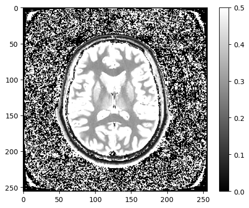
# Simulate a T2-weighted spgr image using the T1 and T2 values voxel-wise, TR = 4000 ms, TE = 100 ms, and FA = 90 degrees
TR = 10000
TI = 3100
TE = 1
FA = 90

flair=ir(1, t1map, t2map, TR, TI, TE, np.deg2rad(FA))

# Plot the T2-weighted spgr image in black and white
plt.imshow(abs(np.rot90(flair)),cmap='gray')
plt.clim(0, 1.2)
plt.colorbar()
plt.show()