Measuring and encoding the MRI signal
1Measuring and encoding the MRI signal
1.1Mathematical Description of Spin System Evolution
Following an excitation of the spin system by an RF energy at the Larmor frequency (γB0), the macroscopic Bloch equation describes how net magnetization evolves over time in a fixed cartesian reference (xi, yj, zk), under B0 is given by:
where M0 is the initial magnetization of the spin system and T1 and T2 are the time constants for the longitudinal and relaxational components of relaxation. The first term of the Equation 2.1 is precessional, and the last two terms are the relaxational components of the Bloch equation. Recall that in thermal equilibrium, the net magnetization is aligned with the applied magnetic field (Figure 2.6c), where the longitudinal component is the net magnetization (M = Mz = M0) and the transverse component equals zero (Mx = My = 0). In this case, the last two terms of the equation vanish, leaving the precessional component of the equation. When the phenomenological Equation 2.1 is solved for the longitudinal (Mz) and the transverse (Mxy) components of the macroscopic magnetization, the explicit solutions are given by:
Note that Equation 2.2 describes an exponential recovery for Mz to return the equilibrium after excitation. On the other hand, Equation 2.3 states that the transverse magnetization follows an exponential decay, quickly converging to zero.
1.2Analogical explanation using a defibrillator
The relationship between the longitudinal and transverse components of magnetization in an NMR experiment can be understood through the analogy of how a defibrillator’s capacitor charges and discharges. As soon as the paramedic hits the shock ⚡️ button, the capacitor abruptly empties to deliver an immediate and strong jolt to the patient (Figure 2.8a). At this moment, the paramedic’s focus is on how the energy dissipates across the patient’s body, which lies in the transverse plane (Mxy). The time it takes from the start of the shock until 37% of the energy remains (1/e = 0.37) corresponds to the T2 time constant of Mxy. This process is very brief, similar to the sound of a click.
After delivering the shock, the capacitor must recharge to the desired level to be ready for the next shock (Figure 2.8b). The time required for the capacitor to reach 63% of its total charge capacity (1-1/e) corresponds to T1 time constant of the Mz. This recharging process is slower and is often accompanied by a rising whine or whirring sound, indicating the gradual buildup of energy.
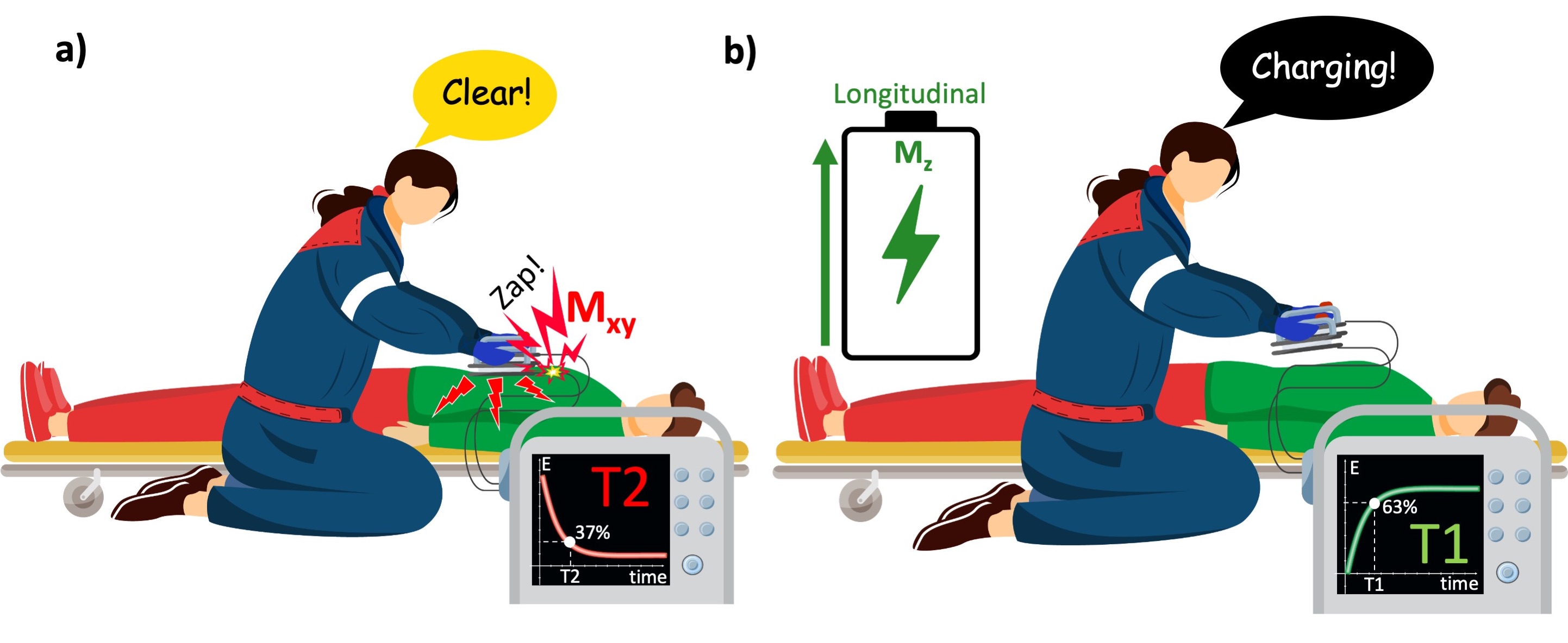
Figure 1:Time-dependent behavior of the transverse and longitudinal magnetization can be compared with how the capacitor of a defibrillator empties and recharges. a) When the paramedic activates the shock paddles, the capacitor quickly discharges its energy to the transverse plane (patient’s body). b) To deliver the shock again, the capacitor must be recharged, which happens quickly, yet relatively much slower than it discharges.
1.3Extending the defibrillator analogy to measurement instrumentation
The use of the defibrillator by a paramedic highlights the distinct nature of T1 and T2 relaxation times in the context of energy dissipation and recovery in a repetitive process. However, it lacks the measurement aspect of an NMR experiment.
To complete the analogy, we will design a calibration setup to measure the energy delivered to the patient’s torso. To measure this indirectly, a loop will be placed under the stretcher and the current induced in the loop as a result of the delivered shock to the patient’s body will be recorded (Figure 2.9). The signal observed at the end of each shock corresponds to the free induction decay (FID) in an NMR experiment.
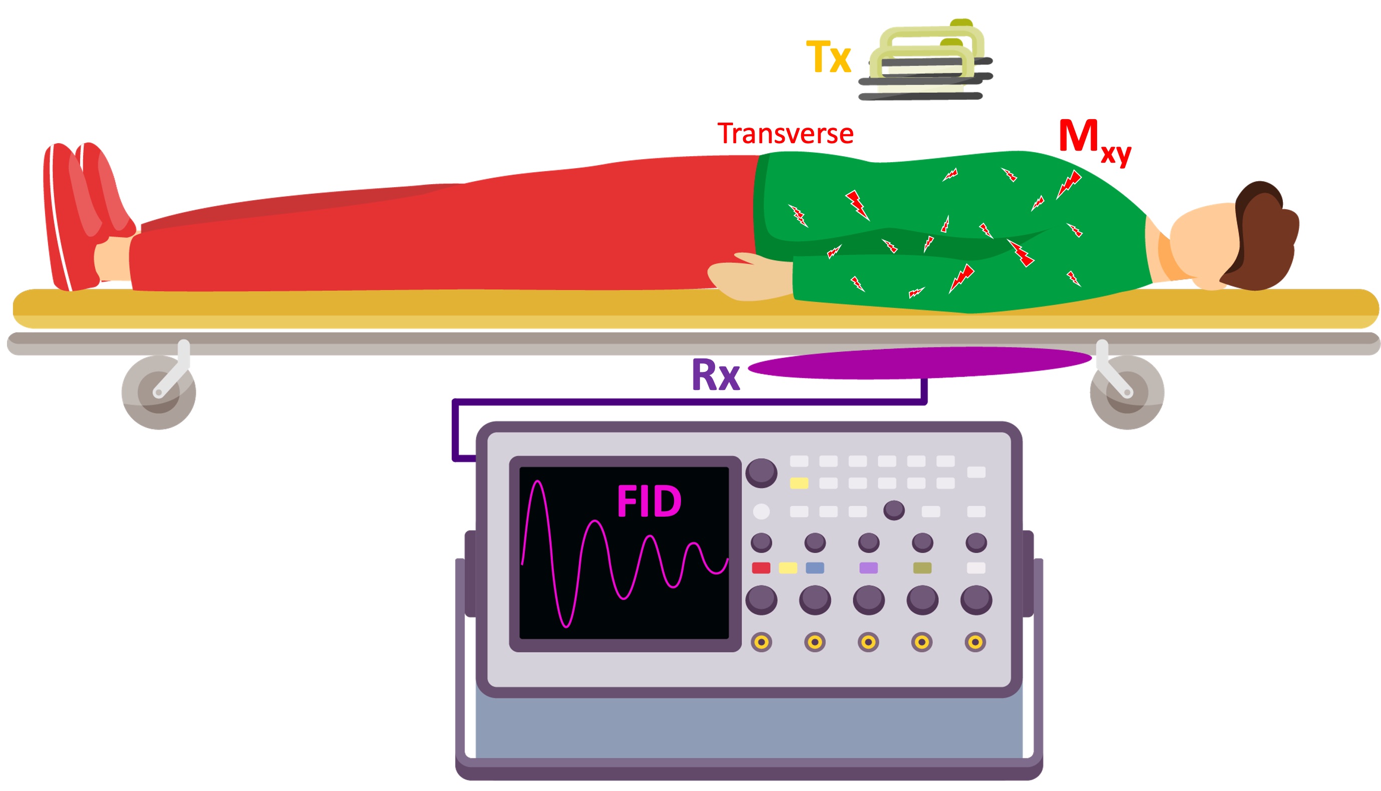
Figure 2:A hypothetical calibration setup: To have a measure of the energy delivered to the patient, a conductive loop is placed under the stretcher. After the shock is delivered, the current induced in the loop is captured by a oscilloscope.
If the biochemical composition of the excited volume varies spatially, the measured FID will be a summation of slightly varying frequency components. For example, a hydrogen atom from the water has a longer response than a hydrogen from the fat (T2fat<T2water). When the frequency components of the FID are observed by applying a Fourier transform, the respective peaks will be separated by a certain extent in the NMR spectrum, depending on the field strength (Figure 2.10).
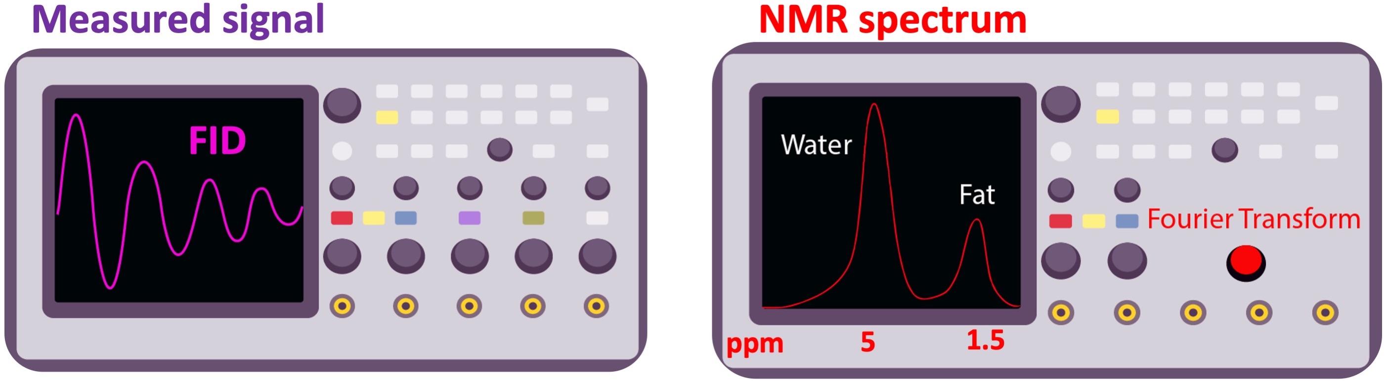
Figure 3:The free induction decay (FID) signal (left), and its frequency spectrum (right). As the electron of the hydrogen atom is more shielded in fat, its peak appears on the lower end (right, by convention) of the chemical shift spectrum. The chemical shift of water and fat is separated by 3.5 part-per-million (ppm), which corresponds to 146 Hz frequency difference at 1T ().
With the ability to precisely reveal molecular signatures, NMR is one of the most popular methods of chemical spectrum analysis, which is still in active use for a broad range of applications. A familiar example would be the benchtop NMR spectrometers at the airports that are used for tracing explosives and narcotics. However, spectral analyses take place in one dimension, in which the application of magnetic resonance was restricted for 25 years.
1.4From the peaks of frequencies to a bright spot in an image: Spatial localization
A magnetic field gradient refers to a gradual change in B0 in any desired direction. This is achieved by flowing high-amplitude electric currents through coils installed in three orthogonal directions. For example, Z gradients (head-foot direction) are a pair of circular Helmholtz coils (green rings in Figure 2.11) that can generate a gradually increasing or decreasing magnetic field by running currents in opposite directions. The higher the current, the steeper the magnetic field difference between the opposite ends of the scanner’s bore. The magnitude of this gradient field can be adjusted such that the spins precess at the Larmor frequency of B0 only at a certain region (selected volume). This way, only the spins from the selected volume will absorb the RF energy deposited at the resonance frequency. To achieve this “spatial localization”, the RF transmitter is turned on concurrently with the gradient coils, sustained briefly (typically in a micro- to milliseconds scale), then turned off. Operating hardware components in this fashion is termed playing (RF or gradient) pulses. Timing of such events is described by pulse sequence diagrams.
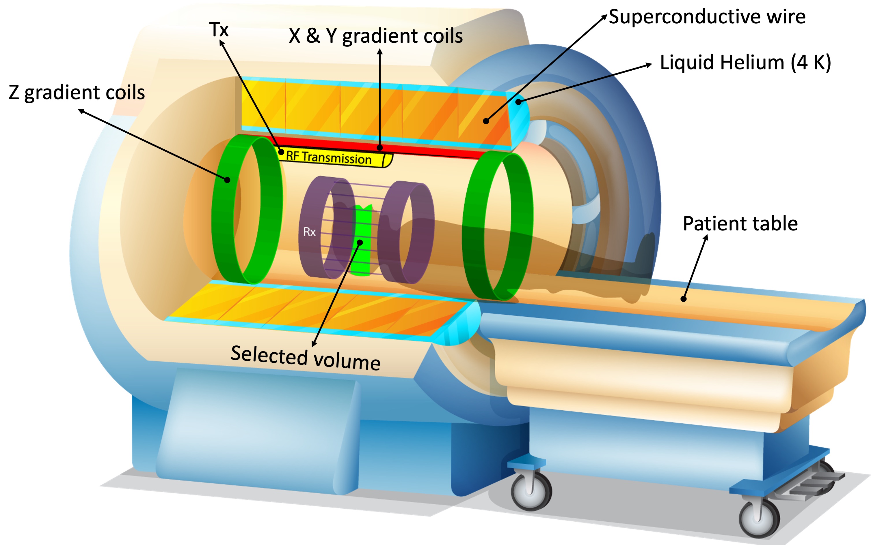
Figure 4:Hardware components of a modern MRI scanner using a superconductive magnet. Z-axis gradients (green rings) spatially vary the magnetic field, such that only the spins at a limited region (light green area in the patient’s head) precess at the Larmor frequency (γB0).
Figure 2.12 shows the sequence diagram describing the spatial localization illustrated in Figure 2.11.
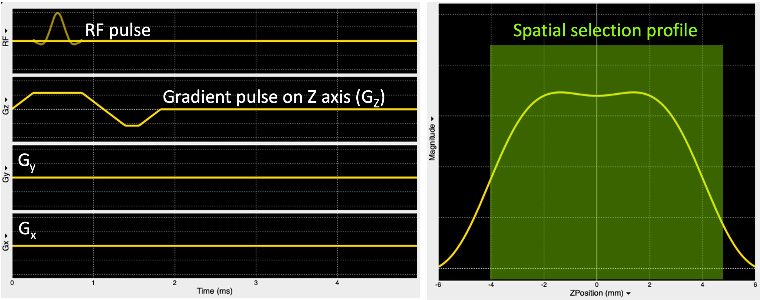
Figure 5:A pulse sequence diagram (left) showing an RF pulse to excite the spins only in a plane selected along the z-axis (Gz) and the respective slice profile (right).
However, the slice selection procedure does not encode the measured signal with positional information. If an ADC event (i.e. signal measurement) was followed soon after the RF pulse was turned off, the receiver coil (Rx, purple, Figure 2.11) would collect information from the whole excited region at once. To form an image, the received signal must be encoded in-plane, which is along the x (row) and y (column) axes (axial plane) for the selected region.
Figure 2.13b explains how spatial encoding in the row direction is performed by playing a gradient along the x-axis (Gx, teal) while the signal is being measured (ADC, purple). As a result of this, spin locations across a single row (the red box outlined in Figure 2.13c) are uniquely sorted out as a function of their frequency, namely the frequency encoding. The process of acquiring data using frequency encoding is termed a readout (purple box) and the acquired data is referred to as an observation (Figure 2.13d). During a readout, the receiver coil picks up a sinusoidal electromagnetic signal as an observation (purple sinusoid in Figure 2.13d), composed of the frequency components encoded per voxel (blue sine waves in Figure 2.13d). Therefore, the ADC must ensure that the observation is sampled at a high enough rate to resolve all 10 frequency components. In this example, the observation must be sampled at least at 20 locations to satisfy the Nyquist condition (purple squares in Figure 2.13d). The ADC hardware of modern MRI scanners is fast enough to achieve high sampling rates up to 500kHz (Graessner, 2013) and smart enough to perform an IQ sampling, separating the magnitude and phase components of each data point (Kirkhorn, 1999). This offers the convenience to place an observation to its location in a special data plane: the k-space (Figure 2.13e).
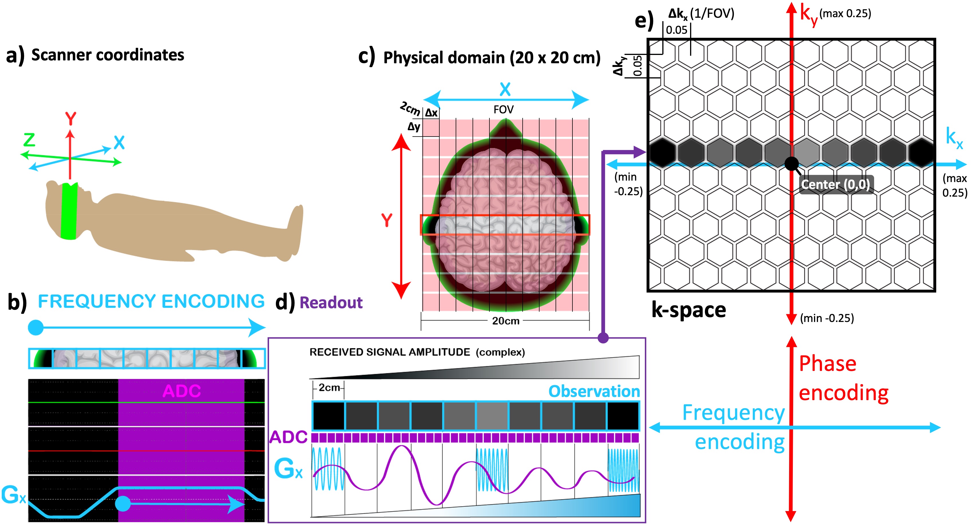
Figure 6:The correspondance between the scanner coordinates (a) and the selected imaging plane (c) is illustrated along with the pulse sequence diagram for frequency-encoding (b). The observation obtained by the readout (d) is shown in the k-space (e).
By convention, the location in the horizontal axis of the k-space is determined by the spatial frequency and the value of each cell is proportional with the magnitude of the respective signal component. The k-space is arranged such that the higher frequency components are located around the skirts, whereas the lower frequency components are closer to the center. In a sense, placing an observation in its k-space location corresponds to adding in the contribution of that acquired portion to the whole image, but in the frequency domain. Hence, there is not a pointwise correspondence between the k-space and the MR image it represents. Instead, every single cell in the k-space (each hexagon in Figure 2.13e) carries information about the whole image. The concept of k-space involves several layers of abstraction that are beyond the scope of this introduction; therefore, the reader is referred to (Mezrich, 1995) for an intuitive understanding of k-space. For the next step of our MR image generation example, we will be concerned with how to fill out multiple rows of the k-space (along the red axis).
Recall that an excitation RF pulse nudges all the spins toward rotating synchronously, so that Mxy across all the pixels share the same phase. Whenever a gradient is played, an opposite effect comes into play: phase of the spins along the gradient direction experiences a location-dependent shift. Each phase shift moves the location of the observation in k-space along the ky axis (Figure 2.14c), upwards or downwards depending on the polarity of the applied gradient. The amount of dephasing (i.e., the number of ∆ky steps) is proportional with the gradient area, and its effect can be rewinded to restore the transverse magnetization by playing a gradient of the same area with opposite polarity. Figure 2.14b shows a phase-encoding gradient (red) played with negative polarity before the readout in order to shift the observation to the next lower row in the kspace (Figure 2.14e). To rewind this dephasing effect, the readout is followed by another Gy gradient with positive polarity.
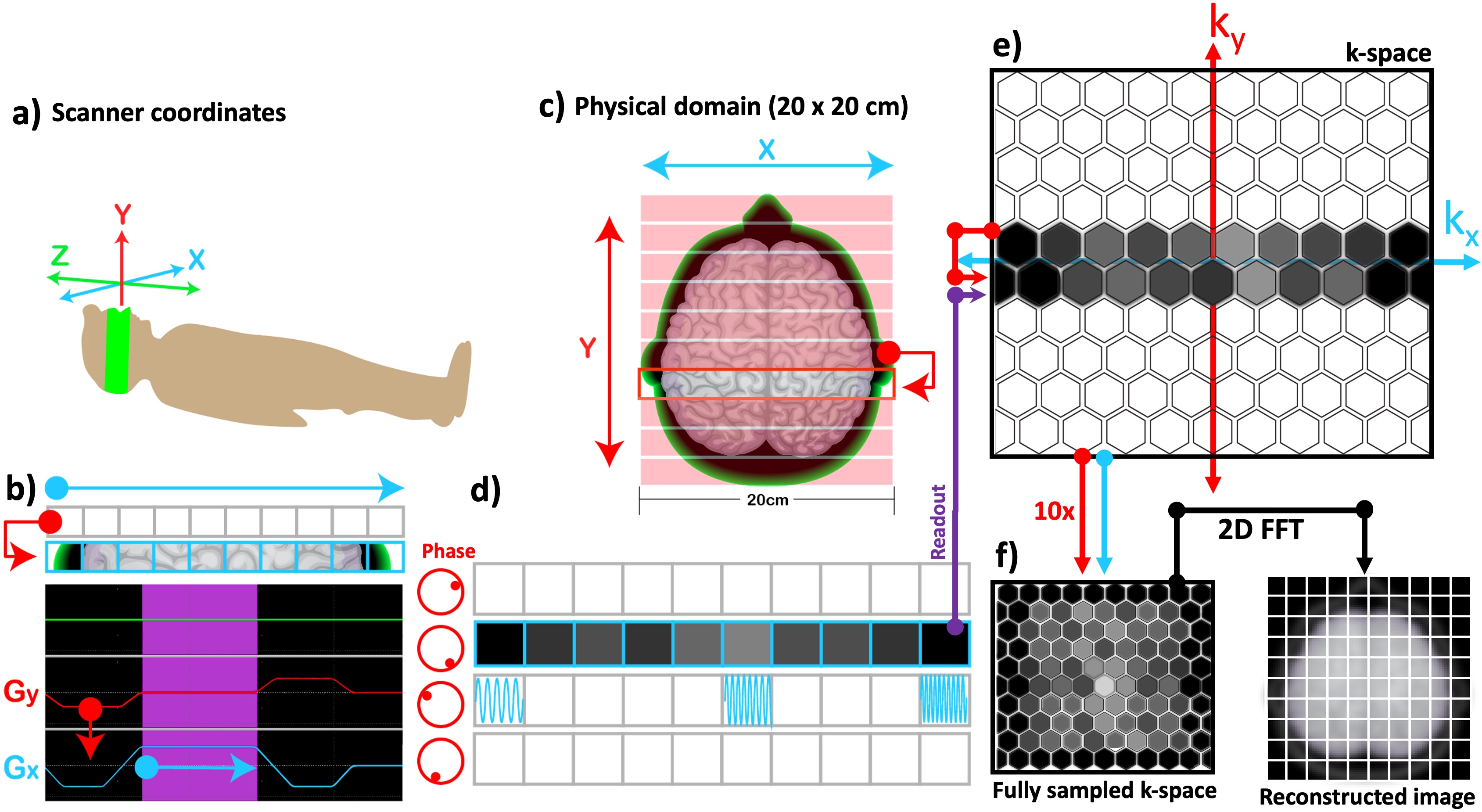
Figure 7:The correspondence between the scanner coordinates (a) and the selected imaging plane (c) is illustrated along with the pulse sequence diagram for phase encoding (b). Once the whole k-space is sampled by incrementing the phase-encoding gradient (red) (b) multiple times, a 2D inverse Fourier transform is applied to reconstruct the MR image (f).
By altering the gradient amplitude stepwise, the whole k-space can be sampled (Figure 2.14f). Therefore, the time that it takes to scan the plane shown in Figure 2.14c is a product of the number of rows and the duration of each repetition, namely the repetition time (TR). Finally, the MR image is reconstructed by applying a 2D inverse Fourier transform to the fully sampled k-space, where each sample corresponds to a grid location.
For the sake of simplicity, the examples in Figure 2.13 and 2.14 assumed that the signal ob- servations followed by an excitation pulse can be used to form an image. However in practice, an FID signal is short-lived; therefore, it cannot directly contribute to reconstructing an MR image. This brings us to two milestone discoveries in NMR by Erwin Hahn, which echoed into the beginning of MRI from a quarter-century behind and have become an indispensable part of its everyday use since then: spin- and gradient-echo. For further reading on the history of these methods, the reader is referred to an MRM Highlights interview with Erwin Hahn (Feinberg, 2018).
- Tamir, J. I., Ong, F., Anand, S., Karasan, E., Wang, K., & Lustig, M. (2020). Computational MRI With Physics-Based Constraints: Application to Multicontrast and Quantitative Imaging. IEEE Signal Processing Magazine, 37(1), 94–104. 10.1109/msp.2019.2940062