Two MRI sequences and two qMRI measurements
Coming full circle back
1Coming full circle back to two measurements with two pulse sequences
“The Court concluded that MRI machines rely on the tissue NMR relaxations that were claimed in the patent as a method for detecting cancer, and that MRI machines use these [T1 and T2 values] to control pixel brightness...” (GE vs Fonar 1996, U.S. Fed. Cir.)
Although going from values to brightness and back again is a 🐓&🥚 problem, GE could have stood a better chance by defending that the pixel brightness can be used to obtain T1 and T2 values, but T1 and T2 values cannot be directly utilized to obtain pixel brightness by MRI machines. Indeed, T1-weighted and T2-weighted contrasts are primarily determined based on the contribution of T1 and T2 (or neither). Nevertheless, to adjust those contributions, MRI machines use pulse sequences and parameters. This section will introduce two essential sequences, spin-echo and gradient-echo to show how contrasts are determined (conventional MRI) and the values are calculated (qMRI).
1.1Spin Echo and T2 mapping
In their seminal article titled “atomic memory”, Brewer and Hahn introduce the spin-echo (Hahn, 1949) by tapping into an intellectual conflict between the 2nd law of thermodynamics and the time reversal symmetry (Brewer and Hahn, 1984). The discussion is illustrated in Fig. 1 to portray the paradoxical nature of the discussions on the physical phenomenon giving rise to a spin-echo. This is yet another effect exploited by the MRI, without necessarily having a complete understanding of the underlying “hidden order” effect emerging from the microscale interactions. For further reading on the conflict between the time symmetry and the entropy, the reader is referred to a recent blog post (Siegel, 2019).
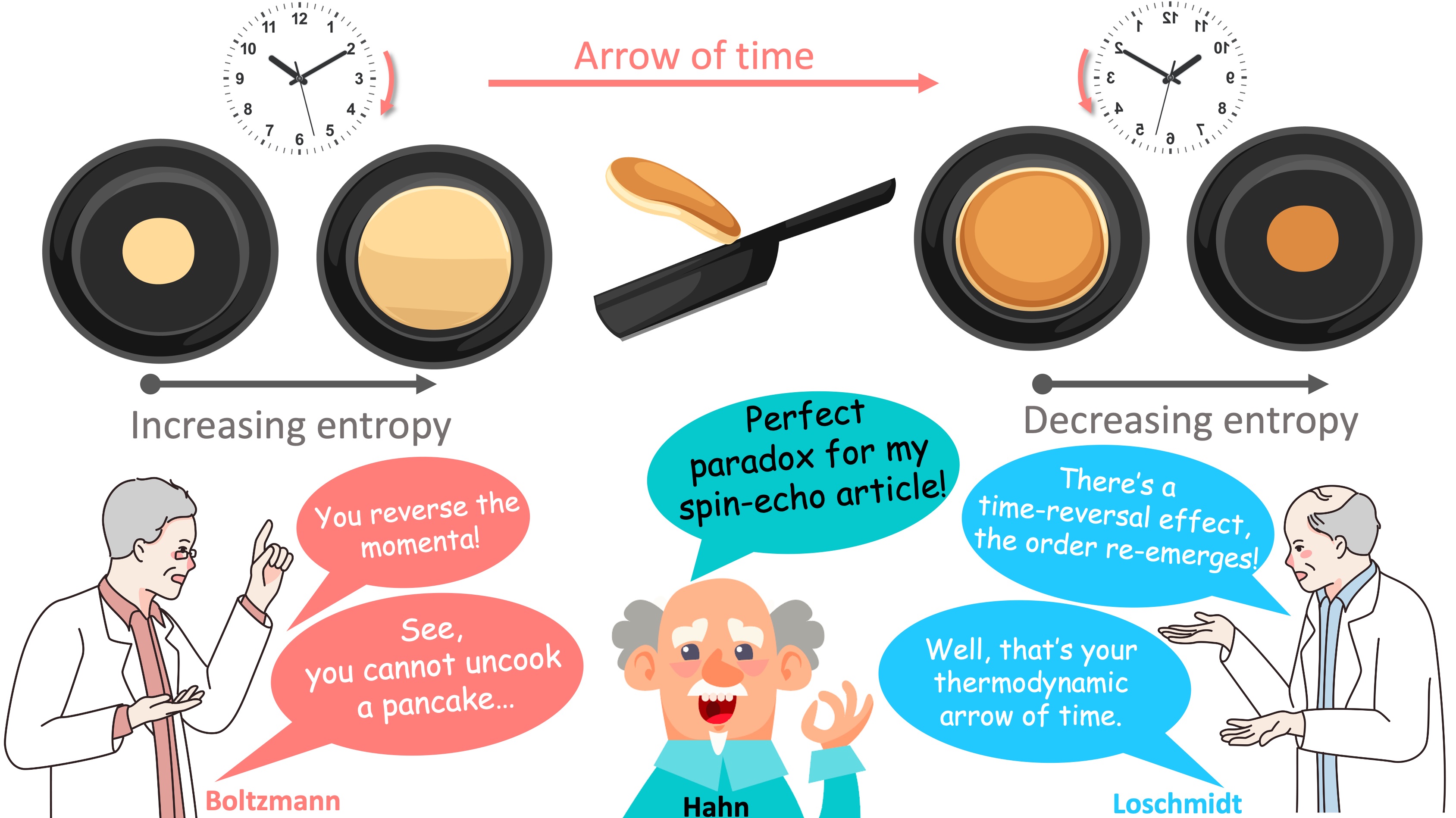
Figure 1:The second law of the thermodynamics (Boltzmann) vs the time reversal symmetry (Loschmidt) and the relation of this conflict to spin-echo (Hahn). The pancake analogy is followed in Fig. 2 for completeness.
Following an excitation pulse, the spin pool goes towards disorderliness and the transverse magnetization decays (the pancake batter expands, Fig. 1). In their article, Brewer and Hahn discuss resurfacing of an ordered state out of this increasing entropy by reversing the phase order of the spins (the cooked pancake contracts). By retaining the pancake analogy, Fig. 2 simulates a spin-echo (SE) pulse sequence and shows the spin evolution at certain time points. At the point (B), a 90°excitation pulse rotates the net magnetization to transfer plane, and after some time, the spins dephase (C, arrows fanning out in the x-y spin scatter plot) as the FID disappears. The “refocusing pulse” rotates the net magnetization by 180°in the transverse plane (D) and reverses the phase order of the spins, analogous to flipping the pancake (Fig. 2). After a period equal to the duration between the 90°and 180°RF pulses, a spin echo is formed (F). The time elapses between the center of the excitation pulse and the peak of the echo signal is termed the echo time (TE).
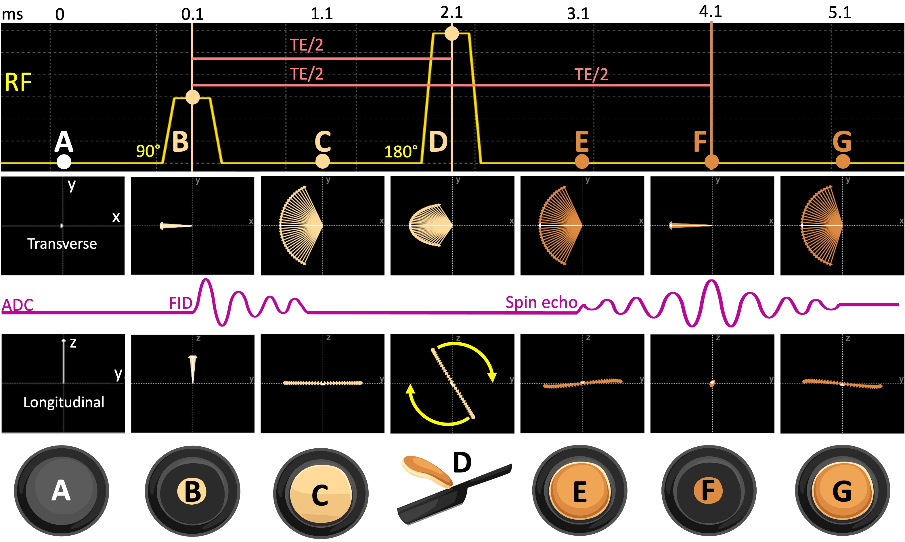
Figure 2:The spin evolution diagram of a spin-echo sequence is shown (A) before the excitation, (B) at the peak of the excitation pulse, (C) one millisecond after the 90°pulse, (D) at the peak of the refocusing pulse, (E) one millisecond after the 180°pulse, (F) at the echo time (TE) and (G) following the echo.
Equation (1) shows the signal representation of a standard SE acquisition. Given that the brightness of the image pixels is determined by the magnitude of the signal S, the relevant contribution of T1 and T2 to the image contrast can be adjusted by changing the TR and TE. For TE → 0 (i.e. short TE), the last term of the equation converges to identity, reducing the T2 contribution. If this is coiled with a long TR (TR → inf), the exponential in the second term of the equation converges to zero, reducing the T1 contribution. Therefore when the TE is short and the TR is long, the contribution to image contrast comes from the density of the spins, i.e. proton density. On the other hand, to increase the T2-weighting by keeping TR the same (long), the TE must be increased (the importance of the last term increases). Fig. 3 exemplifies this by showing the same image across 6 echoes, where substances with longer T2 (e.g., eyes and the cerebrospinal fluid (CSF)) appear gradually brighter compared to the other structures in the image as the TE increases.
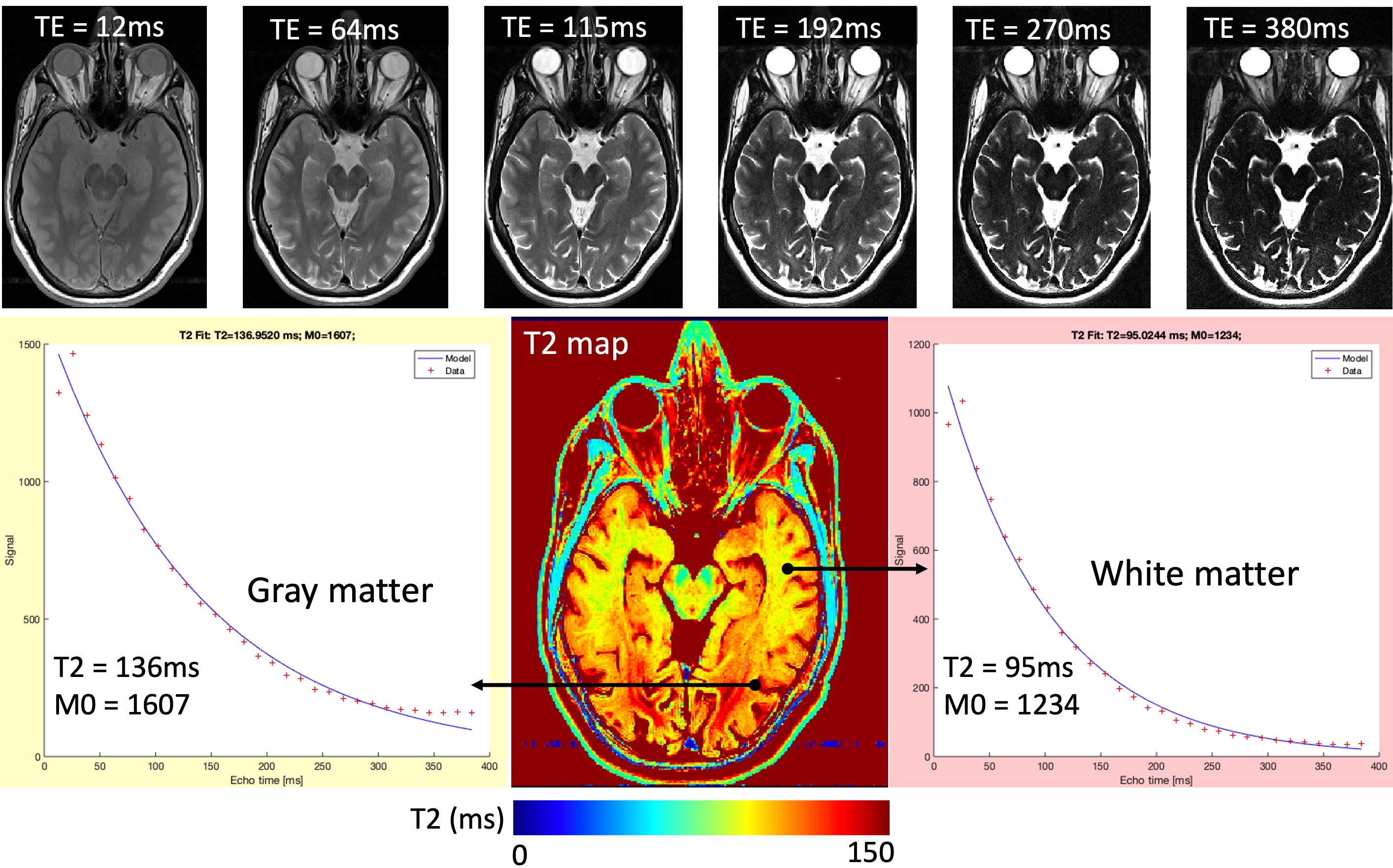
Figure 3:An example T2 map, estimated by fitting voxel-wise brightness values (red plus signs) across 32 echo times to the exponential decay (blue line) defined by Equation (1). The top row shows how conventional image contrast changes from proton-density to T2-weighted as the TE increases from 12ms to 380ms.
Since the signal representation is known for the basic SE acquisition, the signal (the voxel brightness) can be sampled at several TE’s and fitted to the exponential decay defined by the last term of the equation to calculate T2, namely T2 mapping. The second term of the equation will not be taken into account, as the TR will be kept constant across the samples. Fig. 3 shows a T2 mapping example, where an axial image of the human brain was collected across 32 TE’s ranging from 12 to 380ms.
So far we looked at how an echo forms out of a 90-180° pulse pair, and created a T2 map based on its signal representation. Although the images created using SE convey good soft-tissue contrast and are robust against motion artifacts, they often come at the cost of long acquisition time (TR ranges from half to a few seconds) and high RF energy deposition.
1.2Gradient Echo and T1 mapping
Fortunately, MRI offers yet another way to generate echoes by taking advantage of the FID following a single RF pulse. The reversal effect needed for echoing the signal is achieved by dephasing and rephasing the spins with the use of a bipolar gradient (Fig. 4). Therefore, this method is named the gradient echo (GRE).
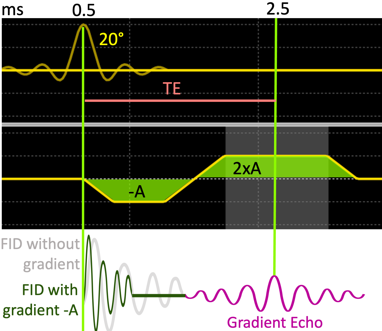
Figure 4:The formation of gradient echo by playing a bipolar gradient followed by a 20°RF pulse.
Unlike SE-based sequences, GRE sequences allow for shorter TE (a few milliseconds) and TR (10-50 milliseconds), resulting in faster acquisitions. In conventional imaging, one of the most popular GRE sequences is the spoiled gradient-echo (SPGR) sequence (Haase et al., 1986), as it allows large volumetric coverage within clinically feasible scan durations. SPGR is also widely used as a basis for various qMRI methods, because it provides a simple signal representation:
Unlike the SE signal representation (Equation (1)), Equation (2) does not include a term explaining the decay of the transverse magnetization by T2. Instead, the last term of the SPGR signal representation indicates that the TE governs the signal contribution of – the effective T2. As the GRE is restored from the FID (Fig. 4), the resulting echo is susceptible to slight variations in the main magnetic field. These variations may originate from the hardware-related imperfections of the B0, or from the field disruptions induced by adjacent substances with distinct magnetization levels, such as the air-tissue interfaces around the nasal cavity. As a result, T2 weighting cannot be achieved with SPGR. Instead, the second term of the Equation 2.5 indicates that the SPGR sequence is primarily T1- weighted, which can be controlled by changing the flip angle (FA) of the excitation pulse (θ) or the TR.
After a number of GRE excitation pulses, the longitudinal magnetization reaches a dynamic equilibrium, i.e. steady-state. When the steady state is reached, the spin system looks static to the observations at a macro-scale, whereas the underlying spin interactions carry on by balancing out each other. This is similar to a person walking up (T1 recovery) an escalator that is going down (the excitation pulse). When this equilibrium is accounted for by the Equation (2), the FA that maximizes the signal for a fixed TR is given by:
where is known as the Ernst Angle (Ernst and Anderson, 1966). Fig. 4 shows this relationship by simulating an SPGR signal across multiple FA at a fixed TR of 30ms for a substance with T1=800ms. It can be seen that the signal is maximized around an FA of 15°, as given by the Equation (3) for these settings (Fig. 5).
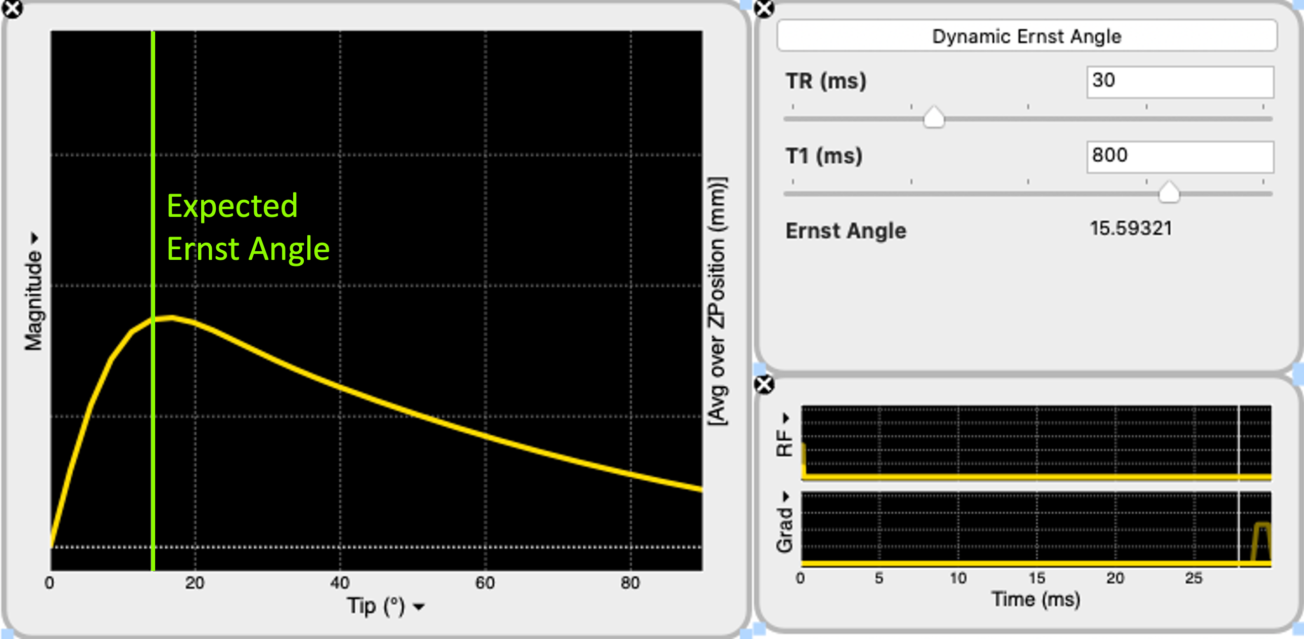
Figure 5:Spoiled gradient-echo (SPGR) signal is simulated for excitation flip angle (FA) ranging from 0 to 90°. With the repetition time set to 30ms, the Ernst Angle () is calculated at 16°for a spin system with T1 of 800ms (Equation (3)). The simulated signal agrees with the calculation, indicating that the signal is the highest when the FA is around 16°(green line).
However, this relationship is valid under the assumption that the transverse magnetization is zero. Therefore, any residual transverse magnetization during the readout violates the steady-state conditions of the signal representation given by Equation (3). To avoid this, the entire spin system is dephased at the end of each TR by using a spoiler gradient, hence the name the “spoiled” GRE. In real-world pulse sequence implementations, the gradient spoiling is coupled with RF spoiling by phase cycling the excitation from TR to TR at predetermined increments (Zur et al., 1991). Fig. 6 displays Bloch simulation results, indicating the critical role of selecting the spoiler gradient area (a), enabling RF spoiling (b) and the selection of a proper phase increment value in disrupting the residual transverse magnetization. The effect of spoiling efficiency becomes particularly important when multiple SPGR acquisitions are performed at different flip angles to calculate a T1 map, namely variable flip angle (VFA) method (Fram et al., 1987). This is simply because when the observed data deviates from the expected signal representation (Fig. 6), the fitted parameters become inaccurate. A more theoretical explanation of the VFA T1 mapping method, its accuracy aspects and limitations are explained in the T1 mapping chapter of this MOOC.
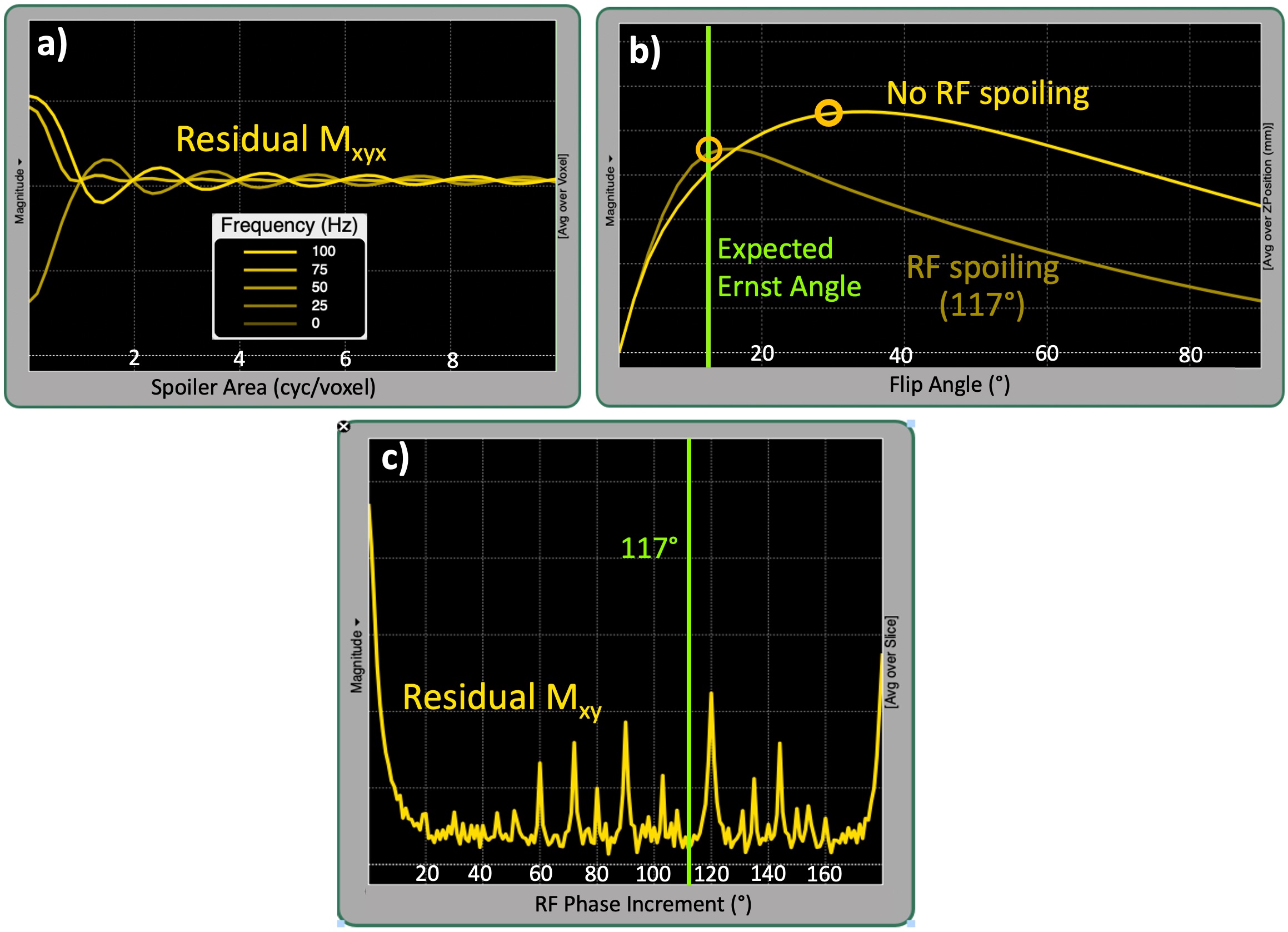
Figure 6:The influence of spoiling on SPGR signal is simulated for (a) the spoiling gradient area ranging from 0 to 10 (cyc/voxel), (b) enabling/disabling RF spoiling at 117° quadratic phase increment and (c) different phase increment values ranging from 0 to 180°.
Fig. 7 shows an example T1 mapping application using the SPGR sequence in a phantom with known values. The acquisitions were performed at two flip angles of 20° (a) and 6° (b), and TR=32ms. Both images show the center of a plate accommodating 14 spheres with T1 values ranging from 0.1 to 1.99 seconds in clockwise ascending order (R1 to R10). In agreement with the Equation 2.4, the image acquired at the higher FA shows superior T1 contrast (a), as the pixel brightness varies inversely with the reference T1 values (d). On the other hand, spheres in the lower FA image show similar brightness (b), in proportion with the spin density of the spheres. From this image pair, a T1 map (c) was estimated using a linear fit as described in (Mathieu), exhibiting good accuracy across the reference values.
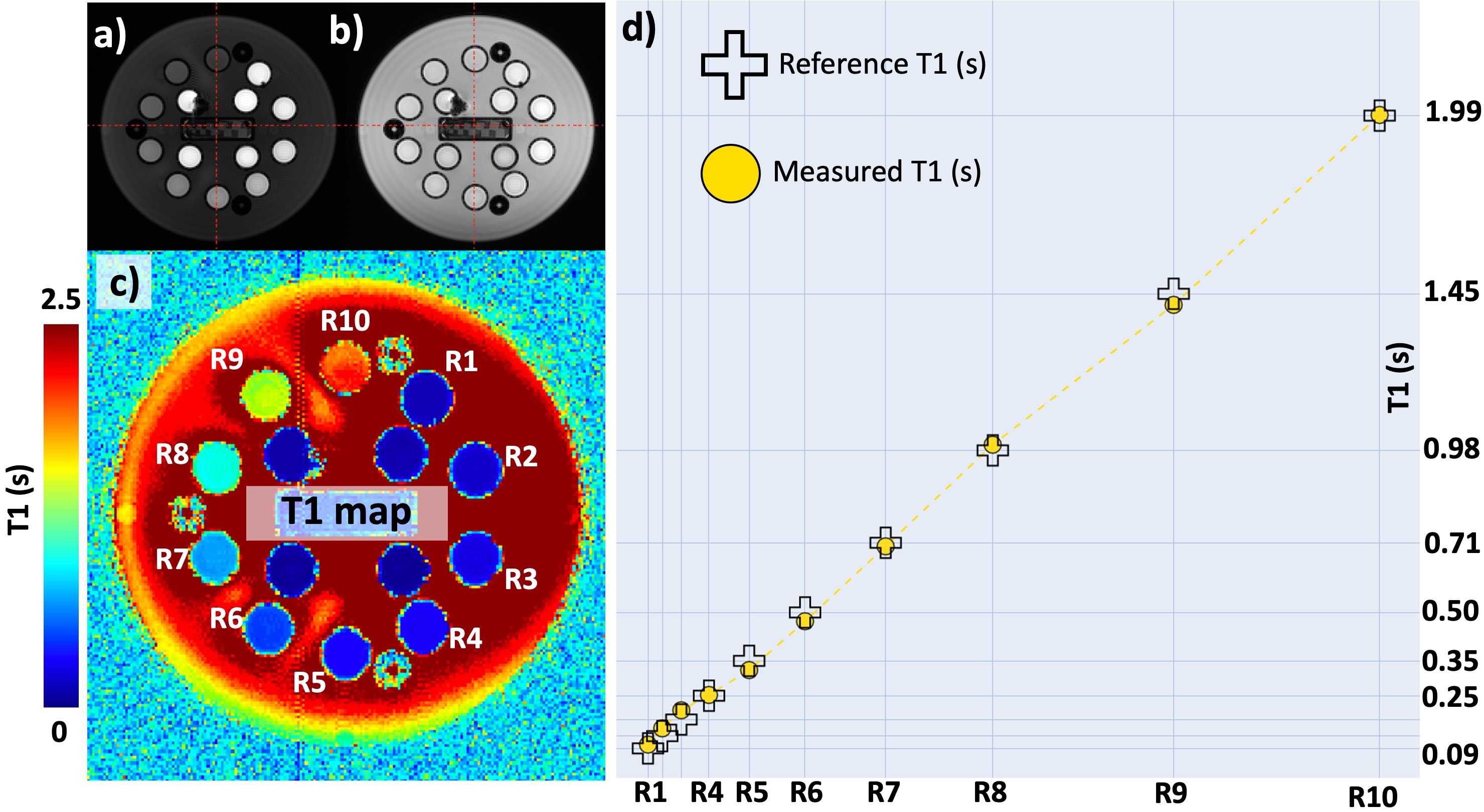
Figure 7:Variable flip angle (VFA) using SPGR sequence. a) T1-weighted and b) PD- weighted images of ISMRM/NIST system phantom acquired at 18 and 32ms, respectively. c) T1 map estimated by fitting images (a) and (b) to the relaxational component of the Equation 2.5. d) The comparison of the estimated and reference T1 values.
In this section, we covered two fundamental pulse sequences: SE and SPGR. Starting from spin-level interactions, we looked at the signal representations of each sequence and how acquisition parameters are associated with the contrast characteristics of the resulting con- ventional images. By doing so, we analyzed how pixel brightness emerges from two values, T2 and T1. Then using the same signal representations, we came full circle back (in case you were wondering what it meant) to these values from the pixel brightness by applying two fundamental qMRI methods, multi-echo SE for T2 and VFA for T1 mapping. A more entertaining summary of the SE and GRE sequences is unintentionally delivered by two indie rock albums (Fig. 8).

Figure 8:Two (slightly modified) album covers by the Artic Monkeys and the Districts summarizing spin-echo (SE) and spoiled gradient-echo (SPGR) sequences.