Appendix B
Magnetization Transfer Saturation
So far we’ve explored a lot of the practical properties of MTsat, but have yet to explore what this parameter represents in reality. We begin this discussion by looking at how Helms et al., 2008 interpreted MTsat:
(figure or quote)
Thus, MTsat is interpreted as being the saturation (i.e. reduction in longitudinal magnetization) occurring from the pulse substituting the MT pulse (Figure 6.15 ) occurring within a single TR, after steady-state has been reached. A reminder: MTR, in contrast, is a steady-state image difference metric (not “within” a TR).
1Simulating MTSat through qMRLab
To assess the validity of this MTsat interpretation, we employ Bloch simulations via qMRLab. These simulations should allow us to visualize the “MTSat value” both as it approaches and after reaching steady-state by quantifying the difference in longitudinal magnetization before and after the MT pulse. The main question we have is: can we find the MT saturation (δ) value directly using Bloch simulations, and how close does it approach the calculated MT saturation value from a three-measurement experiment (equations 7-9)?
Using some high-school geometry, we see how we can calculate MTsat (delta) from this difference, assuming (as Helms did) that the MT saturation causes a flip of a specific angle.
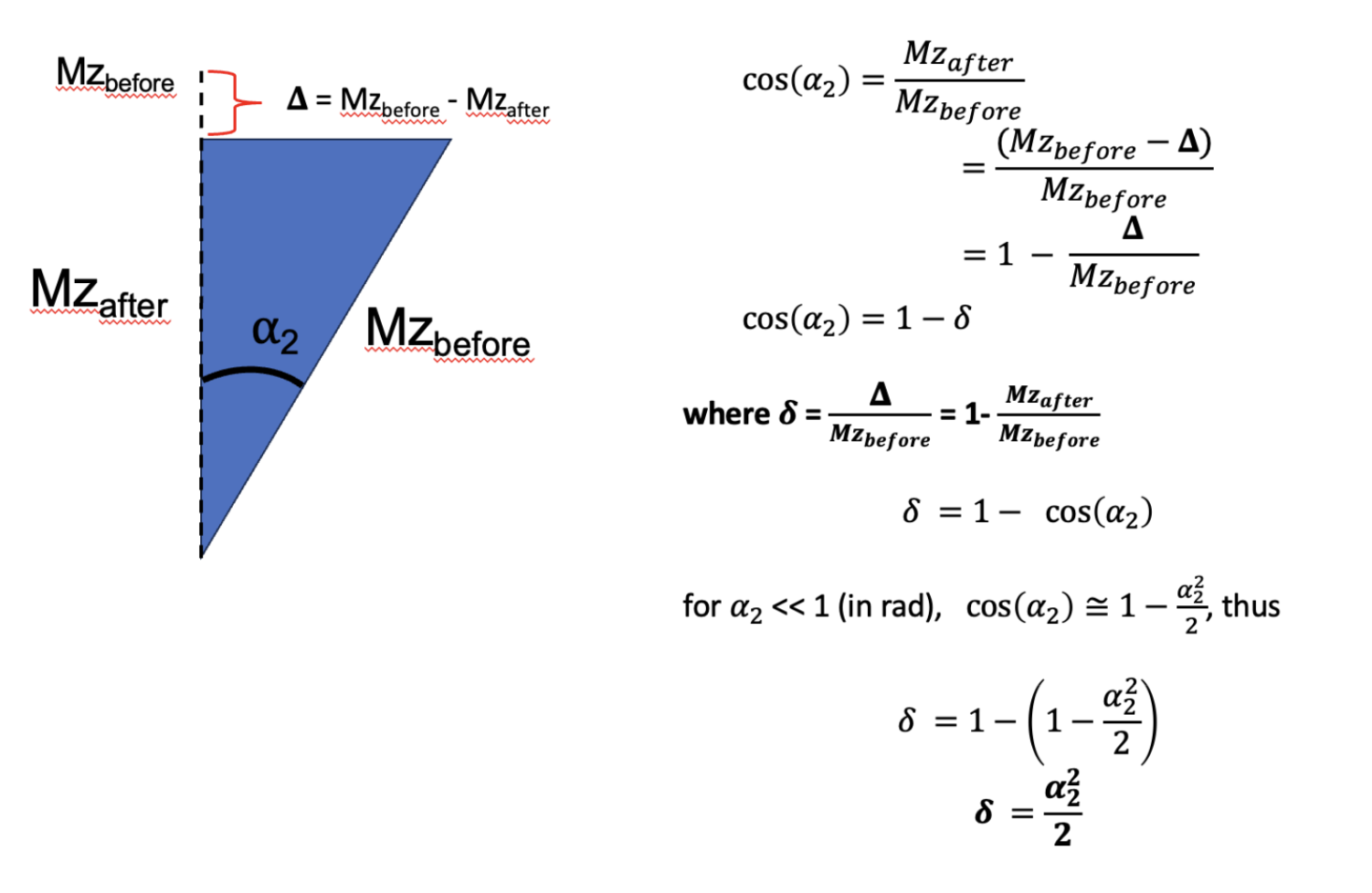
Figure 6A.1:Demonstration through trigonometry of how following a small flip angle alpha2 (eg MT saturation), the value represents the fraction of the reduction in longitudinal magnetization due to the pulse (bigDelta) relative to the value prior to the pulse (Mzbefore).
2Simulation 1: Revisiting MTsat Theory
In our first simulation, we use the qMRLab qMT-SPGR module to simulate steady-state signals from an MTsat experiment on healthy white matter tissues. We utilize tissue parameters from Sled & Pike, 2001 and an MTsat protocol derived from Karakuzu et al., 2022.
Code
clear all, close all, clc

%% Load protocol

fname = 'configs/mtsat-protocols.json';
fid = fopen(fname);
raw = fread(fid,inf);
str = char(raw');
fclose(fid);
val = loadjson(str);

protocols = val.karakuzu2022.siemens1

%% Load tissues

fname = 'configs/tissues.json';
fid = fopen(fname);
raw = fread(fid,inf);
str = char(raw');
fclose(fid);
val = loadjson(str);

tissue = val.sled2001.healthywhitematter;

%% T1 range

T1_true = 1

%% qMT-SPGR experiment

MTsats = zeros(1,length(T1_true))
MTRs = zeros(1,length(T1_true))
T1s = zeros(1,length(T1_true))


protocol = protocols.pdw

fa = protocol.fa
tr = protocol.tr/1000
te = protocol.te/1000
offset = protocol.offset
mt_shape = protocol.mtshape
mt_duration = protocol.mtduration/1000
mt_angle = protocol.mtangle

Model = qmt_spgr;
Model.Prot.MTdata.Mat = [mt_angle, offset];
Model.Prot.TimingTable.Mat(5) = tr ;
Model.Prot.TimingTable.Mat(1) = mt_duration;
Model.Prot.TimingTable.Mat(4) = Model.Prot.TimingTable.Mat(5) - (Model.Prot.TimingTable.Mat(1) + Model.Prot.TimingTable.Mat(2) + Model.Prot.TimingTable.Mat(3)) ;
Model.options.Readpulsealpha = fa;
Model.options.MT_Pulse_Shape = mt_shape

params = tissue{1}
x = struct;
x.F = params.F.mean;
x.kr = params.kf.mean / x.F;
x.R1f = 1/T1_true;
x.R1r = 1;
x.T2f = params.T2f.mean/1000;
x.T2r = params.T2r.mean/(10^6);

Opt.SNR = 1000;
Opt.Method = 'Bloch sim';
Opt.ResetMz = false;

[FitResult, Smodel] = Model.Sim_Single_Voxel_Curve(x,Opt); % NOTE: this uses a modified version of the qmt_spgr.m file where the additional output is included. Not all version of qMRLab has this; if yours doesn't, go to the file and add the additional function output accordingly.

%% Cleanup

%Smodel is the normalized MT-SPGR value, that is, the signal with the MT
%pulse on divided by the signal from the same sequence with the MT pulse
%off. Since in the MTsat experiment, the PD-weighted pulse sequence is the
%latter case above, we then define:

Signal_MT = Smodel;
Signal_PDw = 1;

%% Find scaling value for T1w signal


% Get PDw/T1w ratio from analytical

PDw_Model = vfa_t1;

params.EXC_FA = protocols.pdw.fa;
params.T1 = T1_true; % Could improve by caclulating T1meas from qMT values
params.TR = protocols.pdw.tr/1000; % ms

PDw_anal = vfa_t1.analytical_solution(params);

T1w_Model = vfa_t1;

paramsT1w.EXC_FA = protocols.t1w.fa;
paramsT1w.T1 = T1_true; % ms
paramsT1w.TR = protocols.t1w.tr/1000; % ms

T1w_anal = vfa_t1.analytical_solution(paramsT1w);

T1wPDw_ratio = T1w_anal/PDw_anal

%% Cleanup

% Since Signal_PDw = 1, then it's clear that

Signal_T1w = T1wPDw_ratio

%% Calculate MTsat from signals

Model = mt_sat;
FlipAngle =  protocols.pdw.fa;
TR =  protocols.pdw.tr/1000;
Model.Prot.MTw.Mat = [ FlipAngle TR ];
FlipAngle = protocols.t1w.fa;
TR =  protocols.t1w.tr/1000;
Model.Prot.T1w.Mat = [ FlipAngle TR];
FlipAngle =  protocols.pdw.fa;
TR =  protocols.pdw.tr/1000;
Model.Prot.PDw.Mat = [ FlipAngle TR];

data = struct();
data.MTw=Signal_MT;
data.T1w=Signal_T1w;
data.PDw=Signal_PDw;
FitResults = FitData(data,Model,0);
MTsats = FitResults.MTSAT
MTRs = FitResults.MTR
T1s = FitResults.T1
Output
MTsats =

    5.3428


MTRs =

   58.9758


T1s =

    1.0100
Our results closely align with expectations (T1 fitted ~= T1 input, MTR ~58, MTsat ~5%). Converting the MTsat value to ɑ2 (see [#mtsatFig3]), we find that the MTSat value corresponds to an equivalent excitation pulse of approximately 18.7 degrees. Through Helms’ interpretation, we infer that the MT pulse should be reducing the longitudinal magnetization by roughly 0.05 (ie Mz_after pulse - Mz_before pulse = 0.05).
3Simulation 2: Challenging MTSat Model Assumptions
Using the qMRLab Bloch simulations, we can calculate the difference in longitudinal magnetization before and after the MT pulse, and see if this corresponds to the MTsat value calculated above.
Let’s do that.
Code
Some modifications of the qMRLab code are needed to output the before/after magnetizations into a file.
clear all, close all, clc

%% Load Mz before and after for each TR

load('sim2.mat')

%% Plot Mz before and after for each TR

figure()
plot(Mz_before, 'r')
hold on
plot(Mz_after, 'b')
legend('Mz_{before}', 'Mz_{after}')

figure()
plot(Mz_before(end-10+1:end), 'r')
hold on
plot(Mz_after(end-10+1:end), 'b')
legend('Mz_{before}', 'Mz_{after}')

figure()
plot(1-Mz_after./Mz_before)
legend('1-Mz_{after}/Mz_{before}')

figure()
plot((1-Mz_after./Mz_before)*100)
legend('1-Mz_{after}/Mz_{before}')
From these simulations, we find that there is a 0.314% reduction in longitudinal magnetization before/after the MT pulse after a steady state is achieved, which is an order of magnitude smaller than the MTsat value we calculated earlier for this protocol and tissue parameters (~5%). Either the MTsat theory is wrong, or we’re missing something. Revisiting the pulse sequence ([#mtsatFig1]) and the MTsat model ([#mtsatFig2]), we notice that while the MTsat model assumes instant excitation for both pulses, in reality the MT pulse is relatively long (~10 ms, [#mtsatProtocolTable]). So, while there is a decoupling between MT saturation and relaxation in the MTsat model ([#mtsatFig2]), in reality (and in our simulations) there is relaxation occurring during the MT pulse, and we didn’t account for that in the above simulation.
4Simulation 3: T1 Correction During MT Pulse
In our third simulation, we account for the T1 relaxation during the MT pulse. To simplify the calculations, and like Helms did, we’ll assume a decoupling between the MTsaturation and relaxation and calculate the T1 relaxation recovery independently for the duration of the MT pulse. We’ll then remove this contribution from the Mzafter-Mzbefore we calculated earlier (0.314%).
Code
Some modifications of the qMRLab code are needed to output the before/after magnetizations into a file.
clear all, close all, clc

%% Load Mz before and after for each TR

load('sim2.mat')

%% Plot Mz before and after for each TR

figure()

figure()
plot((1-Mz_after./Mz_before)*100)
hold on
plot((1-(Mz_after-delta_Mz_T1relax)./Mz_before)*100)

legend('MTsat before T1 correction', 'MTsat after T1 correction')

figure()
plot((1-(Mz_after-delta_Mz_T1relax)./Mz_before)*100)
legend('1-Mz_{after}/Mz_{before}')
Upon excluding the T1 contribution, the disparity Δ in Mz values prior to and following the MT pulse increased to 2.1%, which is to say, that the MT contribution of this pulse leads to a reduction of Mz by 2.1%. This outcome aligns with the expected behavior, as T1 relaxation perpetually seeks to increase longitudinal magnetization towards its equilibrium value, which inversely impacts Δ. Consequently, the Δ we just calculated within a given TR is now closer to the initial MTsat calculation based on simulated measurements (2.1% compared to 5.34%). Nevertheless, it is apparent that some critical element eludes our simulations since we’ve only calculated only half of the anticipated value using our Bloch simulations.
5Considering Exchange and Relaxation after the MT Pulse
Once again, let’s compare the actual pulse sequence (Figure 6.14) and the Helms model (Figure 6.15 . In the MTsat model, all of the magnetization exchange contribution is concentrated into the second instantaneous excitation-saturation pulse . In the actual pulse sequence and in our Bloch simulations (Figure 6.14), there is exchange during the MT pulse (which we’ve calculated above), but also when the MT pulse is off (because the longitudinal free and restricted magnetizations are not at equilibrium - see Bloch-McConnell equations in our qMT blog post). So, it’s likely that the contribution of MT when the off-resonance pulse is off also needs to be accounted for, if we want to calculate the MTsat value directly within a TR in Bloch simulations. This additional MT exchange between the restricted and free pool likely causes a reduction in longitudinal free relaxation which is encapsulated in the MTsat value (which makes sense, from the diagrams of the two-pool model of MT).
6Simulation 3: MT contribution after the off-resonance pulse
To calculate this second contribution, we will calculate the difference in Mz between the end of the MT pulse and the end of TR (just prior to the next MT pulse), and just like we did earlier, we’ll also subtract the T1 component (assuming that MT and T1 are decoupled during this time). Note that MTsat is the reduction in magnetization relative to its value prior to the MT pulse, so we need to normalize this contribution by the initial Mz (the same one we used for the MT pulse contribution, at the start of TR). Appendix C extends the diagram from Figure 8 to include the MT contribution after the MT pulse, and although more complex, it demonstrates the need for the note in the previous sentence.
Code
Some modifications of the qMRLab code are needed to output the before/after magnetizations into a file.
clear all, close all, clc

%% Load Mz before and after for each TR

load('sim2.mat')

%% Plot Mz before and after for each TR

figure()

figure()
plot((1-(Mz_after-delta_Mz_T1relax)./Mz_before)*100)

hold on
plot((1-(M0_remainingTR_free-delta_Mz_T1relax_remaining)./Mz_before)*100)
plot((1-(Mz_after-delta_Mz_T1relax)./Mz_before)*100+(1-(M0_remainingTR_free-delta_Mz_T1relax_remaining)./Mz_before)*100)

legend('MTsat contribution from MT pulse event', 'MTsat contribution from cross-relaxation event', 'Total MTsat for TR')
These simulations show through Bloch simulations that the sum of the MT contribution during and after the off-resonance pulse (with the T1 relaxation component removed) leads to a reduction in longitudinal magnetization of 5.49%, very close to the 5.34% that was calculated using the Helms model of MTsat in Eq. 6.7, Eq. 6.8, and Eq. 6.9. A slight overestimate still remains, but this difference is likely impossible to consolidate, as there will always be a difference between the actual MT exchange (where both MT and T1 are counteracting each other at all times) and the modeled MTsat exchange (where instantaneous pulses are assumed, so the MT and T1 contribution are completely separated in this theory).These simulations should however show that the MTsat contribution is not restricted to only the difference in Mz resulting after the effects of the MT pulse, but also to the cross-relaxation occurring between pools in the absence of the MT pulse.
7Interpreting MTSat
In conclusion, our reevaluation of MTSat suggests that it does not model solely the fractional saturation due to the MT pulse within a single TR, as conventionally understood. Instead, MTsat appears to represent the fractional saturation arising from the entire MT contribution during a TR, that is to say, both the MT pulse and the subsequent MT exchange between the two pools that takes place after following the off-resonance pulse. This subtle reinterpretation may challenge existing interpretations, as a greater contribution results from the exchange after the MT preparation pulse due to cross-relaxation caused by the perturbing MT pulse. This analysis highlights the power of open-source qMRI tools like qMRLab in fostering deeper understanding within the field.
Through a meticulous examination of MTSat, we encourage the scientific community to engage in further discussions and research, potentially leading to more refined models and insights into this crucial aspect of MRI physics in modelling tissue components that are difficult to measure directly, such as the semi-solid myelin sheets.
- Helms, G., Dathe, H., Kallenberg, K., & Dechent, P. (2008). High-resolution maps of magnetization transfer with inherent correction for RF inhomogeneity and T1 relaxation obtained from 3D FLASH MRI. Magn. Reson. Med., 60(6), 1396–1407.
- Sled, J. G., & Pike, G. B. (2001). Quantitative imaging of magnetization transfer exchange and relaxation properties in vivo using MRI. Magn. Reson. Med., 46(5), 923–931.
- Karakuzu, A., Biswas, L., Cohen-Adad, J., & Stikov, N. (2022). Vendor-neutral sequences and fully transparent workflows improve inter-vendor reproducibility of quantitative MRI. Magn. Reson. Med., 88(3), 1212–1228.