Theory
Magnetization Transfer Saturation
MTsat, like MTR and many flavours of quantitative MT, is based on spoiled gradient recalled echo (SPGR) images Haase et al., 1986Sekihara, 1987Hargreaves, 2012 preceded by an off-resonance RF pulse to provide magnetization transfer contrast Wolff & Balaban, 1989Henkelman et al., 1993Sled & Pike, 2000Sled, 2018. Figure 6.14 presents a simplified diagram of this MT-prepared SPGR pulse sequence (imaging gradients are not shown). A standard SPGR sequence (low flip angle [~5-10°], short TR [~10-30ms], and a strong spoiler gradient) are preceded by a long (~10 ms) off-resonance (~1-5 kHz) pulse with a strong peak amplitude (the total pulse has an equivalent on-resonance flip angle of 200°-700°). A smooth shape (e.g. Gaussian or Fermi) is typically used for the off-resonance pulse in order to have a single off-resonance frequency (from Fourier analysis). A strong spoiler gradient is also added between the off-resonance MT-preparation pulse and the on-resonance excitation pulse in order to destroy residual transverse magnetization that may have been created by the off-resonance pulse. Images acquired without MT saturation are acquired using the same timing as this sequence, but with the off-resonance RF pulse either completely off or using a very large off-resonance frequency (e.g. ~30+ kHz).
where A is some proportionality constant (e.g. gyromagnetic ratio, density, coil sensitivity, etc), ɑ is the excitation flip angle, R1 = 1/T1 (assuming a monoexponential longitudinal relaxation curve), and TR is the repetition time. Similarly, an analytical equation for the steady-state signal of a dual-excitation SPGR experiment (Figure 6.15 ) can be derived, and Helms et al., 2008 demonstrated it to be:
where is the imaging excitation flip angle, is the excitation flip angle representing the MT saturation pulse, TR1 is the time between to , TR2 is the time between and the following , and TR = TR1 + TR2.
Eq. 6.9 has three unknowns: A, R1, and . Of these three, is expected to be the most sensitive to macromolecular density via the MT effect, and as such is the parameter that we’d like to calculate or fit using this dual-excitation SPGR model for the MT-prepared SPGR pulse sequence. Although there would be some ways to acquire additional measurements (three unknowns, so at a minimum three measurements are needed) and apply a nonlinear fit to Eq. 6.9 to extract , this method has a long numerical processing time. To shorten the calculation of the parameter maps, Helms et al., 2008Helms et al., 2010 (Helms et al. 2008, 2010) proposed some reasonable assumptions that can be made to simplify Eq. 6.9. The first proposed assumption is that R1TR << 1, which is true when using typical MT-weighted SPGR protocol parameters (TR ~ 0.01-0.05 s) and in the brain at clinical field strengths (T1 ~ 1 s, thus R1 ~ 1 s-1). The same approximation applies to TR1 and TR2, which are shorter than TR. This leads to the removal of all exponential functions in Eq. 6.9, as via the Taylor expansion of the exponential function, exp(x) ~ 1 + x when abs(x) << 1, and the removal of another term via R1TR1R1TR2 ~ 0 when R1TR1 and R1TR2 are both << 1. The simplifications result in
The second approximation is that is small (less than 30 degrees), which is to say that the MT saturation is relatively small. This is expected to be true for the tissue properties of the brain (mostly, myelin), but care must be taken with the planned MT pulse parameters as the MT saturation increases with smaller offset frequency and high peak pulse amplitude. Later, we’ll calculate if this is a reasonable assumption for the calculated . This assumption is integrated into Eq. 6.9 via the Taylor series expansion of the , where for small x (this relationship is true for x < 30 degrees or 0.5 radians). Introducing this approximation in [3] and with the additional simplifications R1TR ~ 0 (from the assumptions above), this results in
Note how the signal no longer has a dependency on the individual TR1 and TR2 values, but only on the full TR. The final approximation is isomorphic to the previous one, but for the imaging excitation RF pulse, that is to say, that is small (less than 30 degrees). This is a controllable approximation, as it is a controllable protocol parameter at the scanner. From this assumption, and (from the Taylor series expansion), so introducing both of these into [4] and simplifying and leads to
The term is the only term that includes an MT effect in Eq. 6.5, and thus will be defined as .
Figure 6.16 demonstrates how δ, which represents MTsat as was defined in Helms et al., 2008, is the fractional reduction in longitudinal magnetization after the MT pulse in the MTsat model illustrated in Figure 6.15 relative to the Mz prior to the pulse. Conventionally, MTsat (δ) is reported in percentage, so .
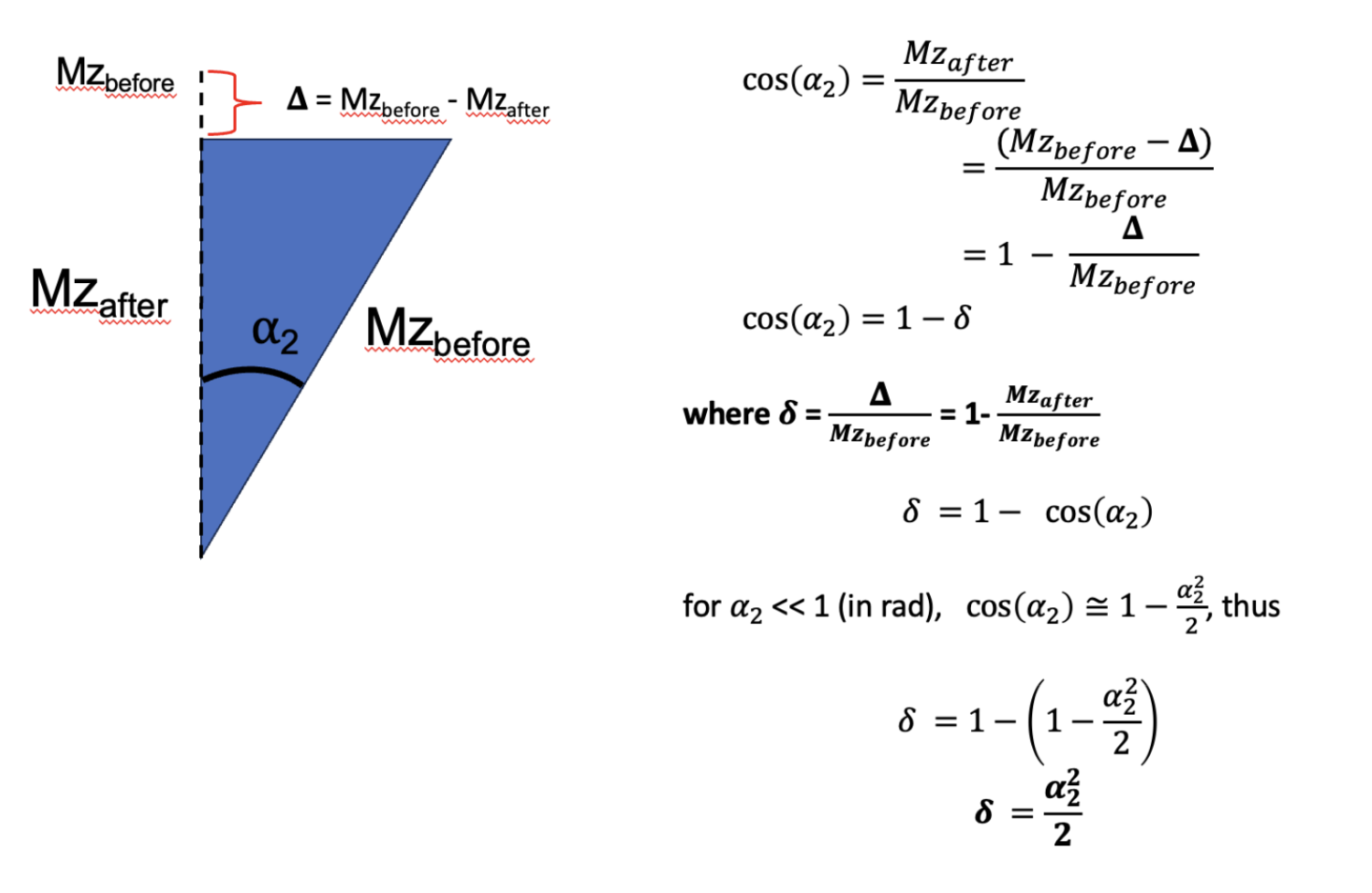
Figure 6.16:Demonstration through trigonometry of how following a small flip angle (eg MT saturation), the value represents the fraction of the reduction in longitudinal magnetization due to the pulse (bigDelta) relative to the value prior to the pulse (Mzbefore).
Before jumping into how to measure MTsat, let’s demonstrate some expected properties and values using known values from a simpler MTR experiment. From the MTR protocol in Brown et al., 2013 of the MTR section, =15 deg and TR = 0.03 s, so assuming a T1 at 1.5T (field strength that Brown used) of 0.55 s in healthy WM, so R1 = 1.8. First off, Figure 6.16 with no MT pulse (thus δ = 0) should converge close to the well-known SPGR equation [1]. Inputting the values in each equations, we get 0.0816A for [1], and 0.0815A, thus they are in close agreement. Next, we can get an estimated value of MTsat, using a known MTR value, the calculated S0 value (which we just did), and then solving [5] for δ using the MTR equation to bring everything together. Doing so is shown in Appendix A, from there and using our simulations in the MTR post with Brown et al., 2013 for healthier WM (MTR = 46%), we get an MTsat value of 4.92% (δ = 0.0492), which is close to some reported MTsat values in the literature (Karakuzu et al. 2022). From there, and by definition of δ, the modeled in Figure 6.15 for this example is 18 degrees, confirming that earlier assumption that < 30 degrees for that approximation.
In that example, we used a known T1 value to extract MTsat using a two-measurement MTR experiment, but in practice this value is not known and varies per-pixel across tissues. Although we could use an additionally measured T1 map to do this, this can be time consuming depending on the method used. (Helms et al. 2008, 2010) thus demonstrated that with one additional T1w measurement that uses no MT preparation pulse but has different /TR than the MTon (MTw) and MToff (PDw) measurements used for MTR, that MTsat can be calculated analytically, and as a bonus a T1 map is also calculated in the process. (This makes sense, as the VFA T1 mapping sequence is often just two SPGR measurements with different α values). Thus, using this three measurement protocol (MTw/PDw/T1w, which we’ll call the MTsat protocol), MTsat and T1 (1/R1) can be calculated analytically pixelwise using the following set of equations (derived from Eq. 6.5):
Remember, like MTR, MTsat is calculated from the equations above following the acquisition of the protocol images; no numerical fitting to a model is required. So effectively, the processing time to produce MTsat maps is the same as MTR, which is nearly instantaneous. Also, unlike MTR, which represents the steady-state signal difference due to the MT effect, MTsat represents the fraction of the longitudinal magnetization saturation caused by a single MT pulse within a TR, after a steady-state is achieved. Conventionally, it is represented as a percentage %, so MTsat is typically reported as . Note that MTR and MTsat are not expected to have the same values in magnitude despite both being represented as %, as they represent different changes. A major benefit of MTsat is that it’s expected to have less T1-dependency than MTR, as T1 (1/R1) is separately calculated and accounted for in the calculation of MTsat using the equations above. Although the MTsat metric is more robust against T1 changes, it is inherently sensitive to the MT preparation pulse properties (due to what MTsat physically represents, which is the saturation due to the MT pulse), and thus MTsat is not truly considered a fully quantitative metric as its value will change depending on the chosen protocol parameters and is not solely specific to the tissue properties or the field properties. Table 6.4 lists some MTsat protocol parameters that have been reported in the literature.
Table 6.4 :Some reported MTsat protocol parameters in the scientific literature (sources: Helms et al., 2008Weiskopf et al., 2013Campbell et al., 2018Karakuzu et al., 2022York et al., 2022)
| Helms 2008 | Weiskopf 2013 | Campbell 2018 | Karakuzu 2022 | York 2022 | |||
|---|---|---|---|---|---|---|---|
| Siemens | Siemens | Siemens | GE | Siemens | Siemens | ||
| T1w | FA | 15 | 20 | 15 | 20 | 20 | 18 |
| TR (ms) | 11 | 18.7 | 11 | 18 | 18 | 15 | |
| TE (ms) | 4.92 | 2.2–14.7 | - | 4 | 4 | 1.54/4.55/8.49 | |
| PDw | FA | 5 | 6 | 5 | 6 | 6 | 5 |
| TR (ms) | 25 | 23.7 | 30 | 32 | 32 | 30 | |
| TE (ms) | 4.92 | 2.2–14.7 | - | 4 | 4 | 1.54/4.55/8.49 | |
| MTw | FA | 5 | 6 | 5 | 6 | 6 | 5 |
| TR (ms) | 25 | 23.7 | 30 | 32 | 32 | 30 | |
| TE (ms) | 4.92 | 2.2–14.7 | - | 4 | 4 | 1.54/4.55/8.49 | |
| Offset (Hz) | 2200 | 2000 | 2200 | 1200 | 1200 | 1200 | |
| MT pulse shape | Gaussian | Gaussian | - | Fermi | Gaussian | Gaussian | |
| MT pulse length (ms) | 12.8 | 4 | - | 8 | 10 | 9.984 | |
| MT pulse angle (deg) | 540 | 220 | 540 | 540 | 540 | 500 | |
- Haase, A., Frahm, J., Matthaei, D., Hanicke, W., & Merboldt, K.-D. (1986). FLASH imaging. Rapid NMR imaging using low flip-angle pulses. J. Magn. Reson., 67(2), 258–266.
- Sekihara, K. (1987). Steady-state magnetizations in rapid NMR imaging using small flip angles and short repetition intervals. IEEE Trans. Med. Imaging, 6(2), 157–164.
- Hargreaves, B. A. (2012). Rapid gradient-echo imaging. J. Magn. Reson. Imaging, 36(6), 1300–1313.
- Wolff, S. D., & Balaban, R. S. (1989). Magnetization transfer contrast (MTC) and tissue water proton relaxation in vivo. Magn. Reson. Med., 10(1), 135–144.
- Henkelman, R. M., Huang, X., Xiang, Q. S., Stanisz, G. J., Swanson, S. D., & Bronskill, M. J. (1993). Quantitative interpretation of magnetization transfer. Magn. Reson. Med., 29(6), 759–766.