Shift function analysis
To run this notebook locally, please make sure that you installed the following libraries by:
install.packages(tibble)
install.packages(png)
install.packages(ggplot2)
install.packages(R.matlab)
install.packages(plotly)
install.packages(htmlwidgets)
install.packages(tidyverse)
install.packages(plyr)
install.packages(dplyr)
install.packages(gridExtra)
install.packages(repr)
install.packages(PairedData)
devtools::install_github('GRousselet/rogme')
install.packages("tidyverse")
Please also set the derivatives directory:
derivativesDir <- "/tmp/VENUS/qMRFlow/"
Note
The following code cell loads all the necessary R libraries and defines some helper functions.
Warning
The data is expected to be found in the /tmp/VENUS directory.
Please do not execute this notebook first. Python notebooks (phantom_python or invivo_python) uses repo2data to download the data on the BinderHub instance. Executing either one of them first will make the data available to this notebook as well.
options(warn = -1)
library(rogme)
library(tibble)
library(ggplot2)
library(R.matlab)
library(plotly)
library(htmlwidgets)
library(tidyverse)
library(plyr)
library(dplyr)
library(png)
library(grid)
library(gridExtra)
library(repr)
library(PairedData)
set.seed(123)

percentage_difference <- function(value, value_two) {
  pctd = abs(value - value_two) / ((value + value_two) / 2) * 100
  return(pctd)
}

obj2plotly <- function(curObj,acq,plim){

if (acq=="rth"){
color="#d62728"
}else{
color="#1f77b4"
}

p<-plot_hsf_pb(curObj, viridis_option="D", ind_line_alpha=0.9, ind_line_size=1, gp_line_colour = "red", gp_point_colour=color,gp_point_size=4,gp_line_size=1.5)
p$labels$colour = ""
p$data$participants = revalue(p$data$participants,c("1"="sub1", "2"="sub2","3"="sub3"))

th <- ggplot2::theme_bw() + ggplot2::theme(
  legend.title = element_blank(),
  axis.line=element_blank(),
    legend.position = "none",
  axis.ticks = element_blank(),
  #axis.text = element_blank(),
  axis.title = element_blank(),
  panel.border = element_rect(colour = "black", fill=NA, size=0.5)
  )

k <-p  + th + aes(x = dec, y = diff, colour = participants) + ggtitle("")

k$labels$colour = revalue(k$labels$colour,c("red"="group"))

axx <- list(
  zeroline = FALSE,
  tickmode = "array",
  tickvals = c("0.1","0.2","0.3","0.4","0.5","0.6","0.7","0.8","0.9"),
  ticktext = c("q1","q2","q3","q4","median","q6","q7","q8","q9"),
  showticklabels= TRUE,
  ticksuffix=" "
)

axy <- list(
  zeroline = FALSE,
  range = c(-plim,plim),
  overlaying = "y2",
  showticklabels= FALSE
  # The range is fixed per panel (3 MAD from both side) to infer the relative effect size
)

axy2 <- list(
  range = c(-plim,plim),
    showticklabels= TRUE,
    ticksuffix=" "
  # The range is fixed per panel (3 MAD from both side) to infer the relative effect size
)
figObj <- ggplotly(k) %>%
            layout(height=800,width=800,xaxis=axx,yaxis = axy, yaxis2 = axy2, margin=c(5,5,5,5)) %>% # SWITCH BACK TO 400 x 400
            style(traces=1,mode="lines+markers",opacity=1,marker=list(size=10),line = list(shape = "spline",color="purple",width=5)) %>%
            style(traces=2,mode="lines+markers",opacity=1,marker=list(size=10),line = list(shape = "spline",color="hotpink",width=5)) %>%
            style(traces=3,mode="lines+markers",opacity=1,marker=list(size=10),line = list(shape = "spline",color="mediumvioletred",width=5)) %>%
            style(traces=4,opacity=1,line = list(color="black",width=2,dash="dash"),yaxis = 'y2') %>% # zero line
            style(traces=5,mode = "lines+markers",opacity=0.9,line = list(shape = "spline",width=3,color="black"),marker = list(color=color,size=30,line=list(color="black",width=1))) %>% # group markers
            style(traces=6,opacity=0,line = list(shape = "spline",color="#762a83",width=3))
return(figObj)
} #END FUNCTION DEF

get_vector <- function(subject, session, metric, nSamples,derivativesDir){
  derivativesDir <- paste(derivativesDir,subject ,"/",sep = "")
  curMat <- readMat(paste(derivativesDir,session,"/stat/",subject,"_",session,"_desc-wm_metrics.mat",sep = ""))
  curMetric <- curMat[[metric]]
  if (metric == "MTR"){
      curMetric <- curMetric[!sapply(curMetric, is.nan)]
      curMetric <- curMetric[curMetric > 35]
      curMetric <- curMetric[curMetric < 70]
  }else if (metric == "MTsat"){
      curMetric <- curMetric[!sapply(curMetric, is.nan)]
      curMetric <- curMetric[curMetric > 1]
      curMetric <- curMetric[curMetric < 8]
  }else if (metric == "T1"){
      curMetric <- curMetric[!sapply(curMetric, is.nan)]
      curMetric <- curMetric[curMetric > 0]
      curMetric <- curMetric[curMetric < 3]
  }
  curMetric <- sample (curMetric, size=nSamples, replace =F)
  return(curMetric)
} #END FUNCTION DEF

get_df <- function(ses1,ses2,metric,nSamples){
df2 <- tibble(participant=as_factor(c(rep(1,nSamples*2),rep(2,nSamples*2),rep(3,nSamples*2))))
df2["condition"] = as_factor(rep(c(rep(ses1,nSamples),rep(ses2,nSamples)),3))
curComp = c(get_vector("sub-invivo1",ses1,metric,nSamples,derivativesDir),
       get_vector("sub-invivo1",ses2,metric,nSamples,derivativesDir),
       get_vector("sub-invivo2",ses1,metric,nSamples,derivativesDir),
       get_vector("sub-invivo2",ses2,metric,nSamples,derivativesDir),
       get_vector("sub-invivo3",ses1,metric,nSamples,derivativesDir),
       get_vector("sub-invivo3",ses2,metric,nSamples,derivativesDir))
df2["metric"] = curComp
return(df2)
} #END FUNCTION DEF

display_sf <- function(derivativesDir,sub,scn1,scn2,metric,implementation){

    T1DIR = paste(derivativesDir,sub,"/","T1_SF_PLOTS",sep="")
    MTRDIR = paste(derivativesDir,sub,"/","MTR_SF_PLOTS",sep="")
    MTSDIR = paste(derivativesDir,sub,"/","MTS_SF_PLOTS",sep="")
    ses_venus=data.frame(row.names=c("G1","S1","S2") , val=c("rth750","rthPRI","rthSKY"))
    ses_native=data.frame(row.names=c("G1","S1","S2") , val=c("vendor750","vendorPRI","vendorSKY"))

    if (metric=="T1"){
        curDir = T1DIR
    }else if (metric=="MTR"){
        curDir = MTRDIR
    }else if (metric=="MTsat"){
        curDir = MTSDIR
    }

    sel1 = ses_venus[scn1,]
    sel2 = ses_venus[scn2,]

    file1 = paste(curDir,"/",sub,"_",sel1,"vs",sel2,"_",metric,"_rev.png",sep="")
    print(file1)
    file2 = paste(curDir,"/",sub,"_",sel2,"vs",sel1,"_",metric,"_rev.png",sep="")

    if (file.exists(file1)){
        plot1 <- readPNG(file2)
        plot2 <- readPNG(paste(curDir,"/",sub,"_",ses_native[scn1,],"vs",ses_native[scn2,],"_",metric,"_rev.png",sep=""))
        grid.arrange(rasterGrob(plot2),rasterGrob(plot1),nrow=1,top=textGrob(label="NATIVE (blue) vs VENUS (red)",size=12))
    }else if (file.exists(file2)){
        plot1 <- readPNG(file2)
        plot2 <- readPNG(paste(curDir,"/",sub,"_",ses_native[scn2,],"vs",ses_native[scn1,],"_",metric,"_rev.png",sep=""))
        grid.arrange(rasterGrob(plot2),rasterGrob(plot1),nrow=1,top=textGrob("NATIVE (blue) vs VENUS (red)"))
    }else {
        print("No file")
    }

}

display_hsf <- function(derivativesDir,scn1,scn2,metric){

    curDir = paste(derivativesDir,"HSF",sep="")
    ses_venus=data.frame(row.names=c("G1","S1","S2") , val=c("rth750","rthPRI","rthSKY"))
    ses_native=data.frame(row.names=c("G1","S1","S2") , val=c("vendor750","vendorPRI","vendorSKY"))

    sel1 = ses_venus[scn1,]
    sel2 = ses_venus[scn2,]

    file1 = paste(curDir,"/",sel1,"vs",sel2,"_HSF_",metric,".png",sep="")
    print(file1)
    file2 = paste(curDir,"/",sel2,"vs",sel1,"_HSF_",metric,".png",sep="")

    if (file.exists(file1)){
        plot1 <- readPNG(file1)
        plot2 <- readPNG( paste(curDir,"/",ses_native[scn1,],"vs",ses_native[scn2,],"_HSF_",metric,".png",sep=""))
        plot3 <- readPNG( paste(curDir,"/",ses_venus[scn1,],"vs",ses_venus[scn2,],"_HSFdif_",metric,".png",sep=""))
        plot4 <- readPNG( paste(curDir,"/",ses_native[scn1,],"vs",ses_native[scn2,],"_HSFdif_",metric,".png",sep=""))
        grid.arrange(rasterGrob(plot2),rasterGrob(plot1),rasterGrob(plot4),rasterGrob(plot3),nrow=2,ncol=2,top=textGrob("NATIVE (blue) vs VENUS (red)"))
    }else if (file.exists(file2)){
        plot1 <- readPNG(file2)
        plot2 <- readPNG( paste(curDir,"/",ses_native[scn2,],"vs",ses_native[scn1,],"_HSF_",metric,".png",sep=""))
        grid.arrange(rasterGrob(plot2),rasterGrob(plot1),nrow=1,top=textGrob("NATIVE (blue) vs VENUS (red)"))
    }else {
        print("No file")
    }

}


derivativesDir <- "/tmp/VENUS/qMRFlow/"

subs = list("sub-invivo1","sub-invivo2","sub-invivo3")
metrics = list("T1","MTR","MTsat")
sessions <- list("ses-rth750rev","ses-rthPRIrev","ses-rthSKYrev","ses-vendor750rev","ses-vendorPRIrev","ses-vendorSKYrev")

options(repr.plot.width=16, repr.plot.height=12)
R.matlab v3.6.2 (2018-09-26) successfully loaded. See ?R.matlab for help.
Attaching package: ‘R.matlab’
The following objects are masked from ‘package:base’:

    getOption, isOpen
Attaching package: ‘plotly’
The following object is masked from ‘package:ggplot2’:

    last_plot
The following object is masked from ‘package:stats’:

    filter
The following object is masked from ‘package:graphics’:

    layout
── Attaching packages ─────────────────────────────────────────────────────────────────────────────────────────────────────────────────── tidyverse 1.3.1 ──
✔ tidyr   1.1.3     ✔ dplyr   1.0.7
✔ readr   2.1.0     ✔ stringr 1.4.0
✔ purrr   0.3.4     ✔ forcats 0.5.1
── Conflicts ────────────────────────────────────────────────────────────────────────────────────────────────────────────────────── tidyverse_conflicts() ──
✖ dplyr::filter() masks plotly::filter(), stats::filter()
✖ dplyr::lag()    masks stats::lag()
------------------------------------------------------------------------------
You have loaded plyr after dplyr - this is likely to cause problems.
If you need functions from both plyr and dplyr, please load plyr first, then dplyr:
library(plyr); library(dplyr)
------------------------------------------------------------------------------
Attaching package: ‘plyr’
The following objects are masked from ‘package:dplyr’:

    arrange, count, desc, failwith, id, mutate, rename, summarise,
    summarize
The following object is masked from ‘package:purrr’:

    compact
The following objects are masked from ‘package:plotly’:

    arrange, mutate, rename, summarise
Attaching package: ‘gridExtra’
The following object is masked from ‘package:dplyr’:

    combine
Loading required package: MASS
Attaching package: ‘MASS’
The following object is masked from ‘package:dplyr’:

    select
The following object is masked from ‘package:plotly’:

    select
Loading required package: gld
Loading required package: mvtnorm
Loading required package: lattice
Attaching package: ‘PairedData’
The following object is masked from ‘package:base’:

    summary
T1, MTR and MTSat shift function analysis
Note
Reproduces Figure 6 from the article for the Participant-3 and includes supplementary analyses for the remaining participants.
The following code cell performs a percentile bootstrapped comparison of dependent samples using Harrell-Davis quantile estimator. Outputs will be written as png and csv files to the following directories:
/tmp/VENUS/qMRFLow/sub-invivo#/T1_SF_PLOTSfor T1 comparisons/tmp/VENUS/qMRFLow/sub-invivo#/MTR_SF_PLOTSfor MTR comparisons/tmp/VENUS/qMRFLow/sub-invivo#/MTS_SF_PLOTSfor MTsat comparisons
Warning
Executing the following code block takes about 10 - 15 minutes per metric!
The outputs are already available in the directories listed above. You can skip the following cell and explore the outputs in the executable Jupyter Lab interface (requires starting a Binder session).
To re-generate the outputs, please un-comment the code block (ctrl or cmd + /).
# metrics = list("MTR","T1","MTsat")
# for (metric in metrics){
# for (sub in subs) {

# T1DIR = paste(derivativesDir,sub,"/","T1_SF_PLOTS",sep="")
# MTRDIR = paste(derivativesDir,sub,"/","MTR_SF_PLOTS",sep="")
# MTSDIR = paste(derivativesDir,sub,"/","MTS_SF_PLOTS",sep="")
# dir.create(T1DIR)
# dir.create(MTRDIR)
# dir.create(MTSDIR)

# sessions <- list("ses-rth750rev","ses-rthPRIrev","ses-rthSKYrev","ses-vendor750rev","ses-vendorPRIrev","ses-vendorSKYrev")

# # Create dataframe with 37k samples per session
# nSamples = 37000
# df <- tibble(N = 1:nSamples)
# for (i in seq(from=1, to=length(sessions), by=1)) {
#   curMat <- readMat(paste(derivativesDir,sub,"/",sessions[i],"/stat/",sub,"_",sessions[i],"_desc-wm_metrics.mat",sep = ""))
#   curMetric <- curMat[[metric]]
#   if (metric == "MTR"){
#       OUTDIR = MTRDIR
#       PLTRANGE = 10.1
#       curMetric <- curMetric[curMetric > 35]
#       curMetric <- curMetric[curMetric < 70]
#   }else if (metric == "MTsat"){
#       OUTDIR = MTSDIR
#       PLTRANGE = 1.7
#       curMetric <- curMetric[curMetric > 1]
#       curMetric <- curMetric[curMetric < 8]
#   }else if (metric == "T1"){
#       OUTDIR = T1DIR
#       PLTRANGE = 0.5
#       curMetric <- curMetric[curMetric > 0]
#       curMetric <- curMetric[curMetric < 3]
#   }
#   # Do not choose the same element more than once
#   print(length(curMetric))
#   curMetric <- sample (curMetric, size=nSamples, replace =F)
#   varName <- toString(sessions[i])
#   varName <- substr(varName,5,nchar(varName)-3)
#   print(varName)
#   df <- mutate(df, !!varName := curMetric)
# }

# neutral = list("rth750","rthPRI","rthSKY")
# native  = list("vendor750","vendorPRI","vendorSKY")
# combns <- combn(c(1,2,3),2)

# for (j in seq(from=1,to=2, by=1)){
# for (i in seq(from=1,to=3, by=1)){

# if (j==1){
#     sel1 = toString(neutral[combns[,i][1]])
#     sel2 = toString(neutral[combns[,i][2]])
#     }
# else
# {
#     sel1 = toString(native[combns[,i][1]])
#     sel2 = toString(native[combns[,i][2]])
# }

# paste(sel1,"vs",sel2," T1",' in progress',sep="")

# grp1 <- df[[sel1]]
# grp2 <- df[[sel2]]

# sfInput <- mkt2(grp1,grp2,group_labels=c(sel1,sel2))
# sf <- shiftdhd_pbci(
#   data = sfInput,
#   formula = obs ~ gr,
#   nboot = 250,
#   alpha = 0.05/30
# )

# sf[[1]]['pctdif'] = percentage_difference(sf[[1]][[sel1]],sf[[1]][[sel2]])
# write.csv(sf,paste(OUTDIR,"/",sub,"_",sel1,"vs",sel2,"_",metric,"_rev",'.csv',sep=""))
# print(min(percentage_difference(sf[[1]][[sel1]],sf[[1]][[sel2]])))
# print(percentage_difference(sf[[1]][[sel1]],sf[[1]][[sel2]])[5])
# print(max(percentage_difference(sf[[1]][[sel1]],sf[[1]][[sel2]])))

# th <- ggplot2::theme_dark() + ggplot2::theme(
#   panel.border = element_blank(),
#   panel.background = element_rect(fill = "black"),
#   plot.background = element_rect(fill = "black"),
#   legend.background = element_rect(fill="white",size=0.5),
#   legend.text=element_text(color="white",size=12),
#   axis.line=element_blank(),
#   axis.text = element_blank(),
#   axis.title = element_blank(),
#   axis.text.x = element_text(colour="white",size=18,face='bold'),
#   axis.text.y = element_text(colour="white",size=18,face='bold')
#   )

# if (j==1){
#     lnclr = "darkgray"
#     flclr = "red"
# } else
# {
#     lnclr = "darkgray"
#     flclr = "blue"
# }

# psf <- plot_sf(
#   data = sf,
#   plot_theme = 1,
#   symb_col = "black",
#   symb_fill = flclr,
#   symb_size = 8,
#   symb_shape = 21,
#   diffint_col = "white",
#   diffint_size = 1.5,
#   q_line_col = "black",
#   q_line_alpha = 0.8,
#   q_line_size = 1.8,
#   theme2_alpha = NULL
# )

# curPlot <- psf[[1]] + geom_hline(yintercept = 0,colour=lnclr, linetype = "longdash",size=1) + ylim(-PLTRANGE,PLTRANGE)
# ggsave(
#   filename = paste(OUTDIR,"/",sub,"_",sel1,"vs",sel2,"_",metric,"_rev",'.png',sep=""),
#   plot = curPlot,
#   device = NULL,
#   path = NULL,
#   scale = 1,
#   width = NA,
#   height = NA,
#   units = c("mm"),
#   dpi = 300,
#   limitsize = TRUE
# )
# }}
# }}
Explore shift function plots
Tip
You can start an interactive BinderHub session to explore VENUS (red) vs NATIVE (blue) shift functions side by side for a selected participant, metric and scanner pairs.
Participants
sub-invivo1sub-invivo2sub-invivo3
Metrics
T1MTRMTsat
Scanners
G1S1S2
subject ="sub-invivo3" # or sub-invivo2 or sub-invivo3
metric ="MTsat" # or MTR or MTsat
scanner1 = "S1" # or S1 or S2
scanner2 = "G1" # or G1 or S2
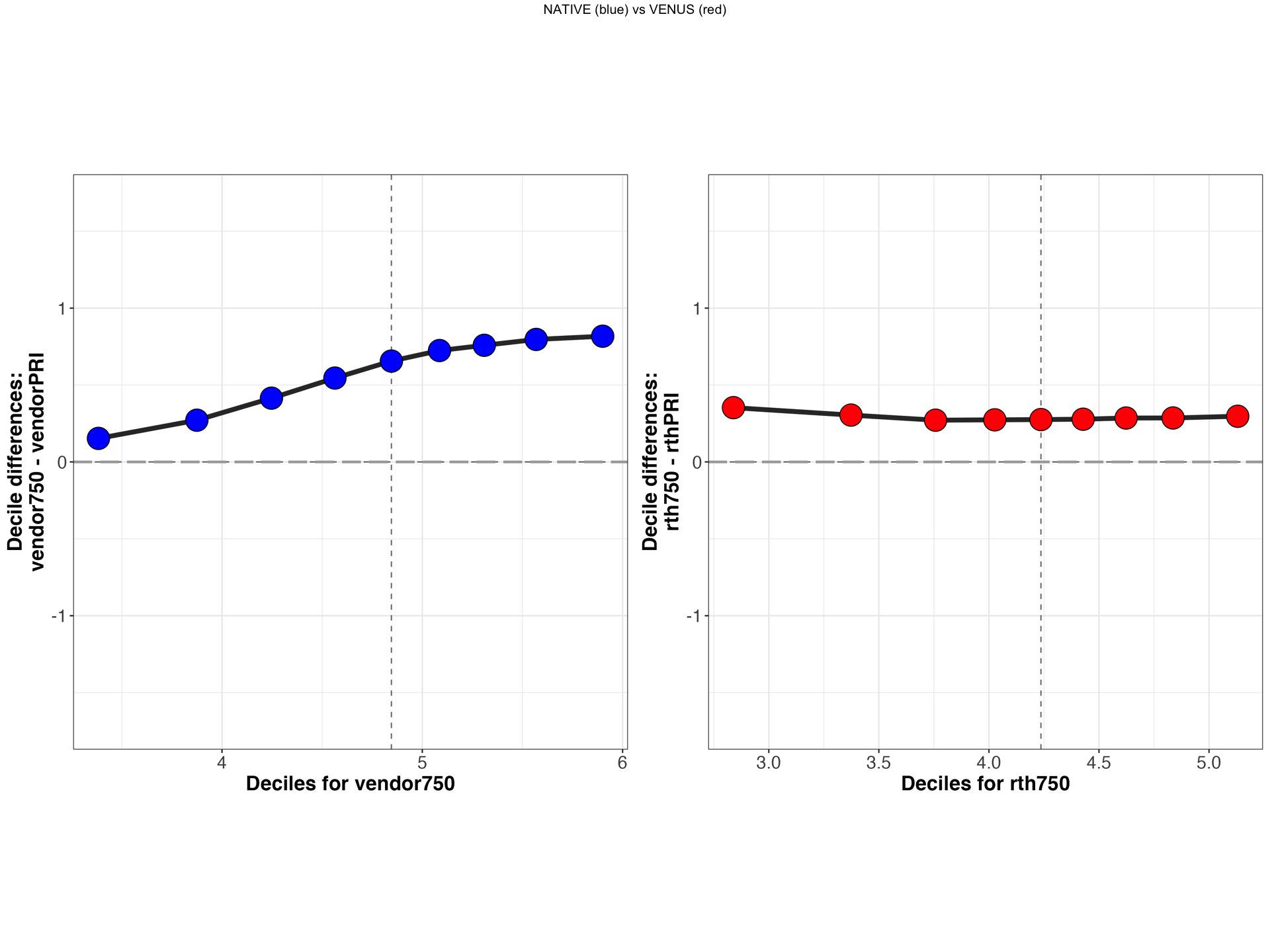
display_sf(derivativesDir,subject,scanner1,scanner2,metric,implementation)
[1] "/tmp/VENUS/qMRFlow/sub-invivo3/MTS_SF_PLOTS/sub-invivo3_rthPRIvsrth750_MTsat_rev.png"
Perform hierarchical shift function (HSF) analysis
Note
Reproduces Figure 7 from the article.
The following code cell iterates over all the comparisons and saves interactive HSF figures.
/tmp/VENUS/HSF
Warning
Executing the following code block takes about 10 - 15 minutes!
The (static) outputs are already available at /tmp/VENUS/HSF. You can skip the following cell and explore the outputs in the executable Jupyter Lab interface (requires starting a Binder session).
To re-generate the outputs and to save interactive plots, please un-comment the code block (ctrl or cmd + /).
You can see interactive visualization from an iteration using
obj2plotly(out,clr,PLTRANGE)
# HSFDIR = paste(derivativesDir,"HSF/",sep="")
# #HSFDIR = paste("HSF/",sep="")
# dir.create(HSFDIR)

# sessions <- list("ses-rth750rev","ses-rthPRIrev","ses-rthSKYrev","ses-vendor750rev","ses-vendorPRIrev","ses-vendorSKYrev")
# nSamples = 37000

# neutral = list("ses-rth750rev","ses-rthPRIrev","ses-rthSKYrev")
# native  = list("ses-vendor750rev","ses-vendorPRIrev","ses-vendorSKYrev")
# combns <- combn(c(1,2,3),2)

# metrics = list("T1","MTR","MTsat")
# for (metric in metrics){

# if (metric == "MTR"){
#       PLTRANGE = 10.3
#   }else if (metric == "MTsat"){
#       PLTRANGE = 1.8
#   }else if (metric == "T1"){
#       PLTRANGE = 0.6
#   }
# for (j in seq(from=1,to=2, by=1)){
# for (i in seq(from=1,to=3, by=1)){

# if (j==1){
#     sel1 = toString(neutral[combns[,i][1]])
#     sel2 = toString(neutral[combns[,i][2]])
#     clr = "rth"
#     }
# else
# {
#     clr = "vendor"
#     sel1 = toString(native[combns[,i][1]])
#     sel2 = toString(native[combns[,i][2]])
# }

# print(paste(sel1,"vs",sel2," T1",' in progress',sep=""))
# cur_df <-get_df(sel1,sel2,metric,nSamples)
# out <- hsf_pb(
#   data = cur_df,
#   formula = metric ~ condition + participant,
#   qseq = seq(0.1, 0.9, 0.1),
#   tr = 0,
#   alpha = 0.05,
#   qtype = 8,
#   todo = c(1, 2),
#   nboot = 750)
# htmlwidgets::saveWidget(obj2plotly(out,clr,PLTRANGE), file = paste(substr(sel1,5,nchar(sel1)-3),"vs",substr(sel2,5,nchar(sel2)-3),"_HSF_",metric,".html",sep=""))
# }}}
Explore HSF plots
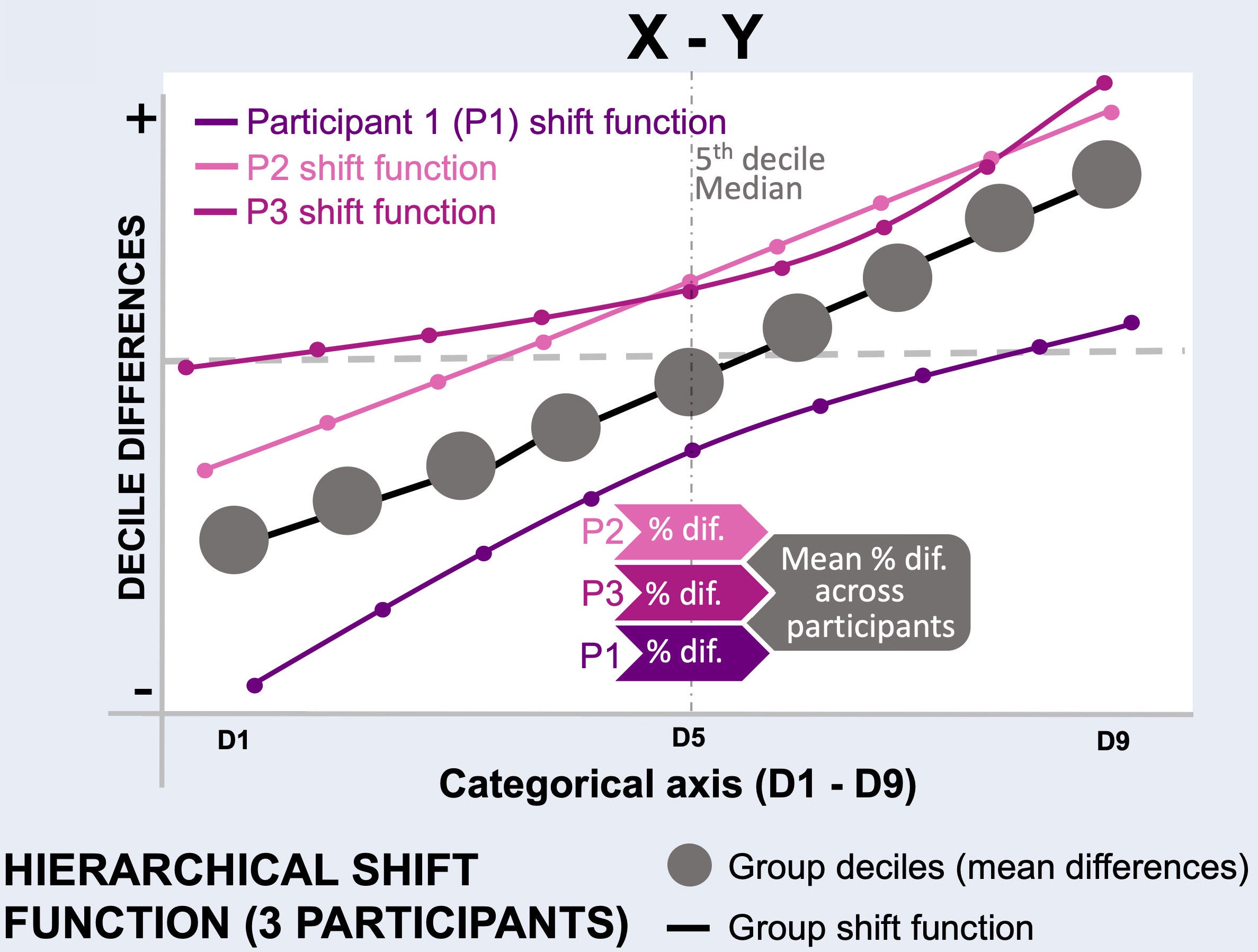
Fig. 5 explanation of the hierarchical shift function analysis.
Tip
You can start an interactive BinderHub session to explore VENUS (red) vs NATIVE (blue) HSF side by side for a selected metric and scanner pairs.
Metrics
T1MTRMTsat
Scanners
G1S1S2
In addition to the HSF plots, respective bootstrapped differences will also be displayed (second row).
metric ="MTsat" # or MTR or MTsat
scanner1 = "G1" # or S1 or S2
scanner2 = "S1" # or G1 or S2


display_hsf("/tmp/VENUS/",scanner1,scanner2,metric)
[1] "/tmp/VENUS/HSF/rth750vsrthPRI_HSF_MTsat.png"
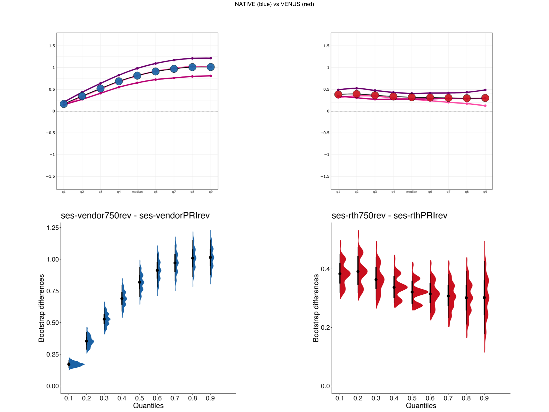
Bootstrapped differences at each decile for HSF
Supplementary
Creates bootstrapped difference plots displayed in the above cell.
# HSFDIR = paste(derivativesDir,"HSF/",sep="")
# dir.create(HSFDIR)

# sessions <- list("ses-rth750rev","ses-rthPRIrev","ses-rthSKYrev","ses-vendor750rev","ses-vendorPRIrev","ses-vendorSKYrev")
# nSamples = 37000

# neutral = list("ses-rth750rev","ses-rthPRIrev","ses-rthSKYrev")
# native  = list("ses-vendor750rev","ses-vendorPRIrev","ses-vendorSKYrev")
# combns <- combn(c(1,2,3),2)

# metrics = list("T1","MTR","MTsat")
# for (metric in metrics){

# if (metric == "MTR"){
#       PLTRANGE = 10.3
#   }else if (metric == "MTsat"){
#       PLTRANGE = 1.8
#   }else if (metric == "T1"){
#       PLTRANGE = 0.6
#   }
# for (j in seq(from=1,to=2, by=1)){
# for (i in seq(from=1,to=3, by=1)){

# if (j==1){
#     sel1 = toString(neutral[combns[,i][1]])
#     sel2 = toString(neutral[combns[,i][2]])
#     clr = "#d62728"
#     }
# else
# {
#     clr = "#1f77b4"
#     sel1 = toString(native[combns[,i][1]])
#     sel2 = toString(native[combns[,i][2]])
# }

# print(paste(sel1,"vs",sel2," T1",' in progress',sep=""))


# cur_df <-get_df(sel1,sel2,metric,nSamples)
# out <- hsf_pb(
#   data = cur_df,
#   formula = metric ~ condition + participant,
#   todo = c(1, 2),
#   nboot = 750)
# obj <- plot_hsf_pb_dist(out,fill_colour=clr,point_interv="median")
# ggsave(
#   filename = paste(substr(sel1,5,nchar(sel1)-3),"vs",substr(sel2,5,nchar(sel2)-3),"_HSFdif_",metric,".png",sep=""),
#   plot = obj,
#   device = NULL,
#   path = NULL,
#   scale = 1,
#   width = NA,
#   height = NA,
#   units = c("mm"),
#   dpi = 300,
#   limitsize = TRUE
# )
# #orca(obj, file = paste(substr(sel1,5,nchar(sel1)-3),"vs",substr(sel2,5,nchar(sel2)-3),"_HSFdif_",metric,".png",sep=""))
# }}}
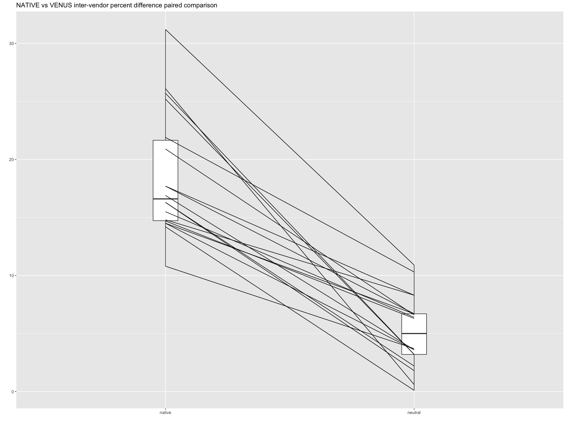
Significance test
Paired comparison of difference scores between VENUS and NATIVE implementations.
Note
The values are drawn from the csv files available at /tmp/VENUS/qMRFlow/sub-invivo#/_SF_ to construct the data frame.
data <- data.frame(participant = rep(1:3, each=12),
                   sequence = rep(c("native","venus"), times=18),
                   metric = rep(c("T1","T1","T1","T1","MTR","MTR","MTR", "MTR","MTsat","MTsat","MTsat", "MTsat"),3),
                   pctdif = c(31.2,10.9,16.30,1.8,17.7,8.3,16.9,3.6,14.5,6.7,25.7,3.2,
                             20.9,6.6,10.8,3.7,15.5,6.4,14.8,8.3,17.7,6.7,25.2,3.2,
                            14.2,0.1,14.5,3.6,14.7,6.3,16.3,2.2,21.9,10.3,26.1,0.6))

# group_by(data, sequence) %>%
#   dplyr::summarise(
#     count = n(),
#     median = median(pctdif, na.rm = TRUE),
#     IQR = IQR(pctdif, na.rm = TRUE)
#   )


neutral <- data$pctdif[data$sequence=="venus"]
native <- data$pctdif[data$sequence=="native"]
pd <- paired(native,neutral)
plt <- plot(pd, type = "profile") + ggtitle("NATIVE vs VENUS inter-vendor percent difference paired comparison") + theme_gray()
# Plotly outputs will not be rendered in Jupyter Book.
# ggplotly(plt)
plt
# Across scores
res <- wilcox.test(pctdif ~ sequence,data=data, paired=TRUE)
p.adjust(res$p.value, method = "BH", n = 6*3)
print('Across metrics significance')
print(res)
# T1
res <- wilcox.test(subset(data,sequence=="native" & metric=="T1")$pctdif,subset(data,sequence=="venus" & metric=="T1")$pctdif,paired=TRUE,alternative = "greater")
print('T1 significance before correction')
print(res)
print('T1 significance after correction')
p.adjust(res$p.value, method = "bonferroni", n = 3)


# MTR
res <- wilcox.test(subset(data,sequence=="native" & metric=="MTR")$pctdif,subset(data,sequence=="venus" & metric=="MTR")$pctdif,paired=TRUE,alternative = "greater")
print('MTR significance before correction')
print(res)
print('MTR significance after correction')
p.adjust(res$p.value, method = "bonferroni", n = 3)

# MTsat
res <- wilcox.test(subset(data,sequence=="native" & metric=="MTsat")$pctdif,subset(data,sequence=="venus" & metric=="MTsat")$pctdif,paired=TRUE,alternative = "greater")
print('MTsat significance before correction')
print(res)
print('MTsat significance after correction')
p.adjust(res$p.value, method = "bonferroni", n = 3)
[1] "Across metrics significance"
	Wilcoxon signed rank exact test

data:  pctdif by sequence
V = 171, p-value = 7.629e-06
alternative hypothesis: true location shift is not equal to 0
[1] "T1 significance before correction"
	Wilcoxon signed rank exact test

data:  subset(data, sequence == "native" & metric == "T1")$pctdif and subset(data, sequence == "venus" & metric == "T1")$pctdif
V = 21, p-value = 0.01563
alternative hypothesis: true location shift is greater than 0
[1] "T1 significance after correction"
[1] "MTR significance before correction"
	Wilcoxon signed rank exact test

data:  subset(data, sequence == "native" & metric == "MTR")$pctdif and subset(data, sequence == "venus" & metric == "MTR")$pctdif
V = 21, p-value = 0.01563
alternative hypothesis: true location shift is greater than 0
[1] "MTR significance after correction"
[1] "MTsat significance before correction"
	Wilcoxon signed rank exact test

data:  subset(data, sequence == "native" & metric == "MTsat")$pctdif and subset(data, sequence == "venus" & metric == "MTsat")$pctdif
V = 21, p-value = 0.01563
alternative hypothesis: true location shift is greater than 0
[1] "MTsat significance after correction"