Signal Modelling
Quantitative Magnetization Transfer
The magnetization transfer in a two-pool model is modelled by a set of coupled differential equations Sled & Pike, 2000:
where the magnetization at time t is given by and and are the transverse magnetization for the free pool in the x and 𝑦 direction, respectively. The longitudinal magnetization for the free and restricted pool is denoted by and . Due to the very short T2 of the restricted pool (on the order of microseconds), the transverse magnetization of this pool is not explicitly modelled.
The constants kf and kr represent the exchange rate of the longitudinal magnetization from the free pool to the restricted pool (kf) and from the restricted to the free pool (kr). The ratio of these quantities is constrained by the size of the restricted to the free-water pool, expressed as . This ratio is called the pool size ratio F defined as . The precessional frequency is a measure of the power of the off-resonance radiofrequency pulse and ∆ is a frequency offset at which the magnetic B1+ field is applied. As shown in Figure 6.1, an on-resonance (∆ = 0) radiofrequency pulse is also part of the pulse sequence and is applied after the MT pulse. The relaxation time constants for the free and restricted pools are denoted by T1,f and T1,r for the longitudinal magnetization, and T2,f and T2,r for the transverse magnetization. Finally, 𝑊 is the saturation rate of the restricted pool, which is a function of the absorption lineshape 𝐺 that depends on the frequency offset and the transverse relaxation of the restricted pool (Figure 6.2).
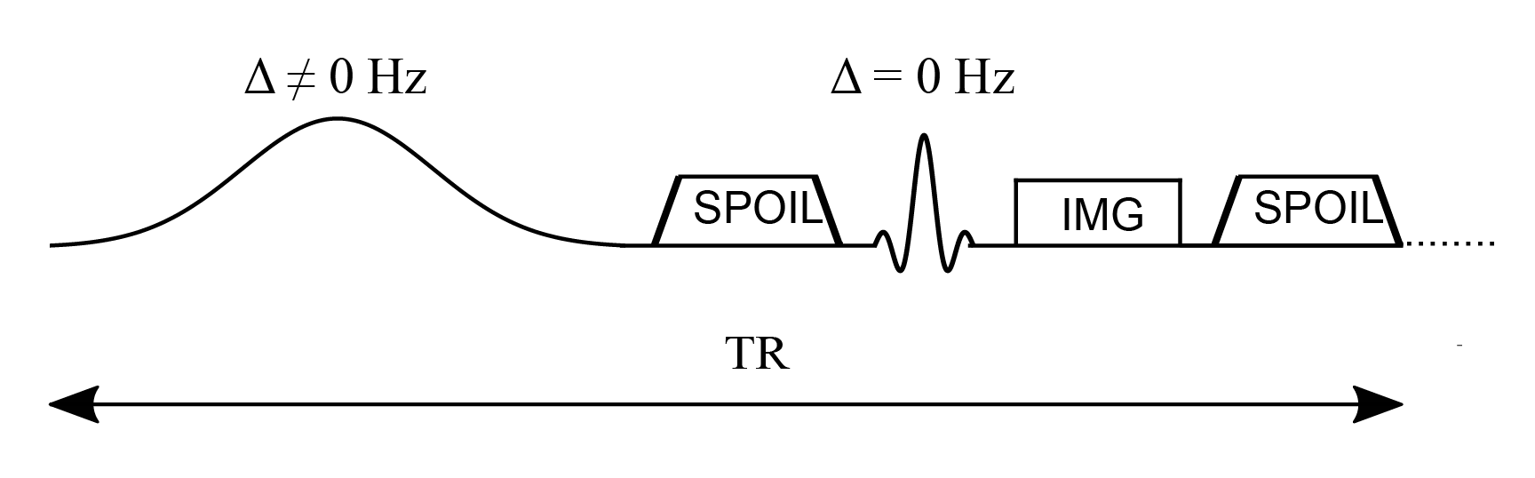
Figure 6.1:Simplified pulse sequence diagram of a magnetization transfer spoiled gradient (MT-SPGR) experiment with an MT pulse followed by a spoiler gradient to destroy any transverse magnetization before the application of the on-resonance excitation pulse.
The absorption lineshape of the restricted pool that best characterizes the proton system depends on the environment. For simple systems such as agar gel phantoms, the Gaussian lineshape describes magnetization transfer effects well Henkelman et al., 1993, while for more complicated and biologically relevant models, the super-Lorentzian lineshape is the best choice Morrison et al., 1995.
Figure 6.2:Gaussian, Lorentzian and super-Lorentzian absorption lineshapes plotted as a function of the frequency offset ∆ and T2,r.
In a standard qMT experiment, multiple measurements are required where the off-resonance radiofrequency pulse angle (MT angle) and offset frequency are changed for each measurement, and at least one measurement is acquired in the absence of an MT pulse. The acquired signal plotted as a function of the the offset frequency is known as the “Z-spectrum”, and Figure 6.3 shows the Z-spectrum simulated using different absorption lineshapes. The off-resonance MT pulse is modelled either as a continuous wave or as a pulsed irradiation scheme. In a continuous wave irradiation mode, long off-resonance pulses of constant saturation and fixed frequency offset are applied to generate well-defined MT states in the two pools Henkelman et al., 2001. For more practical implementations, pulsed off-resonance irradiations are used with a spoiled gradient echo sequence (SPGR) to generate MT-weighted images at different saturation rates and frequency offsets Sled & Pike, 2000. In the qMT-SPGR sequence shown in Figure 6.1, the MT preparation pulse is applied, followed by a spoiler gradient to eliminate any residual transverse magnetization produced by the long MT pulses, and to destroy the MR signal from previous measurements. A signal equation for this type of pulsed MT experiment can be derived by approximating the pulse sequence to a series of stages described by a continuous wave off-resonance irradiation period, followed by free precession, and instant saturation of the free-water pool Cabana et al., 2015Sled & Pike, 2000Sled & Pike, 2001. This pulse sequence decomposition allows for analytically solving the Bloch-McConnell equations at a steady-state, but it is also possible to numerically solve the Bloch equations to perform simulations that provide a more realistic approximation when the system has not been driven to a steady-state. A comparison between the Bloch simulations and the analytical solution is shown in Figure 6.4 for different numbers of preparation MT pulses. As can be seen, different frequency offsets and MT flip angles require different numbers of repetition times to reach the steady-state, which is of paramount importance since the analytical solution used for parameter estimation is derived assuming the steady-state. In terms of data acquisition optimization, the k-space periphery is sampled during the preparation pulses whereas the center of k-space, that contains the overall image contrast, is acquired once the steady-state is achieved.
Figure 6.3:Z-spectrum simulated using different absorption lineshapes (Gaussian, Lorentzian, and super-Lorentzian).
Figure 6.4:Z-spectrum simulated using Bloch simulations (dashed lines) for a number of MT pulses ranging from 1 to 600. Bloch simulations are compared with the Z-spectrum obtained from the analytical solution (solid lines).
- Sled, J. G., & Pike, G. B. (2000). Quantitative interpretation of magnetization transfer in spoiled gradient echo MRI sequences. J. Magn. Reson., 145(1), 24–36.
- Henkelman, R. M., Huang, X., Xiang, Q. S., Stanisz, G. J., Swanson, S. D., & Bronskill, M. J. (1993). Quantitative interpretation of magnetization transfer. Magn. Reson. Med., 29(6), 759–766.
- Morrison, C., Stanisz, G., & Henkelman, R. M. (1995). Modeling magnetization transfer for biological-like systems using a semi-solid pool with a super-Lorentzian lineshape and dipolar reservoir. J. Magn. Reson. B, 108(2), 103–113.
- Henkelman, R. M., Stanisz, G. J., & Graham, S. J. (2001). Magnetization transfer in MRI: a review. NMR Biomed., 14(2), 57–64.
- Cabana, J.-F., Gu, Y., Boudreau, M., Levesque, I. R., Atchia, Y., Sled, J. G., Narayanan, S., Arnold, D. L., Pike, G. B., Cohen-Adad, J., Duval, T., Vuong, M.-T., & Stikov, N. (2015). Quantitative magnetization transfer imagingmadeeasy with qMTLab: Software for data simulation, analysis, and visualization. Concepts Magn. Reson. Part A Bridg. Educ. Res., 44A(5), 263–277.