The pulse sequence of the AFI method (Figure 4.5) is composed of two identical RF pulses and two different delays (TR1 < TR2). After each RF pulse, the signal intensity is acquired followed by a spoiler to destroy the residual transverse magnetization next to the following RF pulse. This method implements a pulsed steady-state signal with a gradient-echo acquisition, thus preventing the use of long repetition times Yarnykh, 2007. It has been demonstrated that if the delays TR1 and TR2 are sufficiently short (e.g. TR1/TR2 = 20 ms/100 ms), and the transverse magnetization is completely spoiled, the ratio of signal intensities (r = S2/S1) depends on the flip angle of applied pulses and is highly insensitive to T1 Yarnykh, 2007.
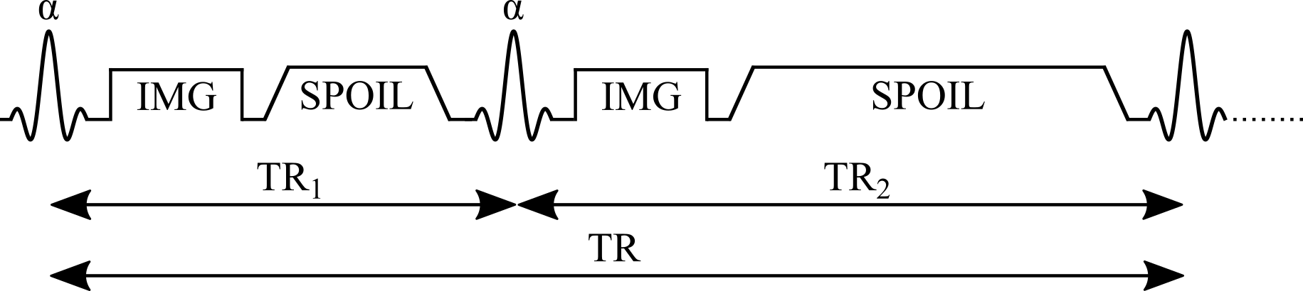
Figure 4.5:Simplified pulse sequence diagram of an actual flip-angle imaging (AFI) pulse sequence with a gradient echo readout. TR1: repetition time 1, TR2: repetition time 2, θ: excitation flip angle for the measurement, IMG: image acquisition (k-space readout), SPOIL: spoiler gradient.
The magnetization of an AFI experiment can be modeled under steady-state conditions by the implementation of a fast repetition of the sequence (TR1 < TR2 < T1). The solution of the Bloch equations for the AFI method is given by Equations 1 and 2 that represent the longitudinal magnetization before the application of the RF pulses:
Mz1,2 is the longitudinal magnetization of both pulses, M0 is the magnetization at thermal equilibrium, TR1 is the delay time after the first pulse, TR2 is the delay time after the second identical pulse (Figure 4.5), and θ is the excitation flip angle. The steady-state longitudinal magnetization Mz curves for different T1 values for a range of and TR values are shown in Figure 4.6.
Figure 4.6:Longitudinal magnetization before the first radiofrequency pulse (Eq. 4.10, solid lines) and before the second identical pulse (Eq. 4.11, dashed lines) for three different T1 values.
The analytical solution of the Bloch equations in a steady-state experiment (Eq. 4.10 and Eq. 4.11) makes several assumptions leading to practical challenges. First, it is assumed that the longitudinal magnetization has reached a steady state after a sufficiently large number of repetition times (TR), and that the transverse magnetization is perfectly spoiled prior to each pulse. To explore these properties, a numerical approach known as Bloch simulations is used to estimate the signal from an MRI experiment given a set of sequence parameters. Here, the Bloch simulations allow us to estimate the magnetization using a different number of sequence repetitions, and look at a special case when the steady-state is not achieved (due to a small number of sequence repetitions). As can be seen in Figure 4.7, the number of repetitions required to reach a steady-state depends on T1 and the flip angle.
Figure 4.7:Signal 1 (blue) and Signal 2 (red) curves simulated using Bloch simulations (solid lines) for a number of repetitions ranging from 1 to 150, plotted against the ideal case (Eq. 4.10 and Eq. 4.11 – dashed lines). Simulation details: TR1 = 20 ms, TR2 = 100 ms, T1 = 900 ms, 100 spins. Ideal spoiling was used for this set of Bloch simulations (transverse magnetization was set to 0 at the end of each TR1,2).
In practice, gradient and RF spoiling are important parameters to consider in an AFI experiment. A combination of both Zur et al., 1991Bernstein et al., 2004 is typically recommended, and Figure 4.8 shows how this better approximates the ideal spoiling case.
Figure 4.8:Signal 1 curves estimated using Bloch simulations for three categories of signal spoiling: (1) ideal spoiling (blue), gradient & RF Spoiling (red), and no spoiling (orange). Simulation details: TR1 = 20 ms, TR2 = 100 ms, T1 = 900 ms, T2 = 100 ms, TE = 5 ms, 100 spins. For the ideal spoiling case, the transverse magnetization is set to zero at the end of each TR. For the gradient & RF spoiling case, each spin is rotated by different increments of phase (2𝜋 / # of spins) to simulate complete dephasing from gradient spoiling, and the RF phase of the excitation pulse is Bernstein et al., 2004 with Zur et al., 1991 after each TR.
- Yarnykh, V. L. (2007). Actual flip-angle imaging in the pulsed steady state: a method for rapid three-dimensional mapping of the transmitted radiofrequency field. Magn. Reson. Med., 57(1), 192–200.
- Zur, Y., Wood, M. L., & Neuringer, L. J. (1991). Spoiling of transverse magnetization in steady-state sequences. Magn. Reson. Med., 21(2), 251–263.
- Bernstein, M., King, K., & Zhou, X. (2004). Handbook MRI Pulse Sequences. Elsevier.