MTR in practice
Magnetization Transfer Ratio
Typically, MTR imaging protocols are implemented on the scanner by adding a relatively long (~5-10 ms) high amplitude off-resonance (~2kHz) preparation RF pulse prior to each TR of an existing imaging sequence. In the early days of MT, the MT pulse was a very long pulse (~10 seconds) prior to one imaging readout of saturation-recovery sequences, but this results in impractically long acquisition times and is very SAR prohibitive. Alternative approaches were explored (eg. 1-2-1 pulses), however now most MT-weighted sequences are done using steady-state sequences (eg SPGR) with a shorter preparation pulse (~10 milliseconds). Figure 6.8 illustrated this using a spoiled-gradient recalled echo (SPGR) sequence, with a Gaussian-shaped MT preparation pulse prior to the excitation pulse.
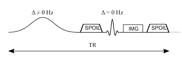
Figure 6.8 :Simplified pulse sequence diagram of an MTR imaging sequence. An off-resonance and high powered MT-preparation pulse is followed by a spoiler gradient to destroy any transverse magnetization prior the application of the imaging sequence, in this case a spoiled gradient recalled echo (SPGR).
Each MRI vendor optimizes their MT-weighted protocol parameters (eg MT shape, duration, frequency, and amplitude), and few of these details are typically shared with the end-user. Table 6.2 shares protocol parameters used by different MRI manufacturers as reported by two publications.
Table 6.2 :Literature MTR protocol parameters (sources: Brown et al., 2013Karakuzu et al., 2022)
| Brown 2013 | Karakuzu 2022 | |||
|---|---|---|---|---|
| Siemens | Philips | GE | Siemens | |
| FA (deg) | 15 | 15 | 6 | 6 |
| TR (ms) | 30 | 47 | 32 | 32 |
| TE (ms) | 11 | 8 | 4 | 4 |
| Offset (Hz) | 1500 | 1100 | 1200 | 1200 |
| MT pulse shape | Gaussian | Sinc-Gaussian | Fermi | Gaussian |
| MT pulse length (ms) | 7.68 | 15 | 8 | 10 |
| MT pulse angle (deg) | 500 | 620 | 540 | 540 |
These differences in protocol parameters can result in MTR values that vary greatly between vendors and sites, meaning that MTR can be challenging to compare unless great care in details are taken. Figure 6.9 shows MTR simulations using the fundamental qMT parameters for four different tissues (Table 6.2 ; healthy cortical grey matter, healthy white matter, NAWM, early white matter multiple sclerosis lesion, late white matter multiple sclerosis lesion) using the four MT-weighted SPGR protocols from Table 6.2 .
Table 6.2 :Quantitative MT parameters in healthy and diseased human tissue reported for a study at 1.5 T Sled & Pike, 2001.
| Healthy cortical GM | Healthy WM | NAWM | Early WM MS lesion | Late WM MS lesion | |
|---|---|---|---|---|---|
| F | 0.072 ± 0.013 | 0.161 ± 0.025 | 0.15 ± 0.02 | 0.12 ± 0.02 | 0.094 ± 0.015 |
| kf | 2.4 ± 0.013 | 4.3 ± 1.0 | 4.9 ± 1.3 | 3.6 ± 0.8 | 2.7 ± 0.7 |
| R1,f (s-1) | 0.93 ± 0.2 | 1.8 ± 0.3 | 1.78 ± 0.4 | 1.52 ± 0.2 | 1.26 ± 0.3 |
| R1,r (s-1) | 1 | 1 | 1 | 1 | 1 |
| T2,f (ms) | 56 ± 8 | 37 ± 8 | 38 ± 7 | 43 ± 6 | 52 ± 9 |
| T2,r (μs) | 11.1 ± 8 | 12.3 ± 1.6 | 11.4 ± 1.4 | 10.3 ± 1.1 | 10.9 ± 1.4 |
Figure 6.9:MTR values calculated from fundamental qMT tissue parameters for four different MTR imaging protocols.
As demonstrated in the above simulations, one MTR value could have the same value for healthy tissue on one scanner as diseased tissue would have on another scanner. So for the most part, MTR is best used / compared within vendors at the very least, though some normalization techniques have been developed.
In addition to being very sensitive to protocol implementations, MTR values are also sensitive to other tissue properties. As seen in the qMT blog post, the parameter most closely related to macromolecular content is the pool-size ratio F. But, if some disease / symptom impacts T1 independently of underlying macromolecular content, MTR will also change. That is to say, MTR is sensitive to tissue’s T1 value independently of the macromolecular content metric F, as shown in Figure 6.10.
Figure 6.10:MTR value for (protocol?) and (tissue?) changes as a function of the underlying T1 value (T1,obsobs or T1,f?).
In addition to being sensitive to tissue properties, MTR is also sensitive to system properties such as B1 (via MT pulse amplitude) and B0 (via off-resonance frequency). In particular, B1 can vary up to 30% the nominal value at 3T, and without correction this can introduce substantial Figure 6.11 illustrates how MTR can vary with different B1 values.
Figure 6.11:MTR value for (protocol?) and (tissue?) changes as a function of the underlying B1 value (T1,obsobs or T1,f?).
Lastly, MTR is sensitive to protocol adjustments, which could be done by a scanner operator to accommodate issues during an imaging session. Figure 6.12 demonstrates how MTR varies with TR adjustments.
Figure 6.12:MTR value for (protocol?) and (tissue?) changes as a function protocols TR value.
- Brown, R. A., Narayanan, S., & Arnold, D. L. (2013). Segmentation of magnetization transfer ratio lesions for longitudinal analysis of demyelination and remyelination in multiple sclerosis. Neuroimage, 66, 103–109.
- Karakuzu, A., Biswas, L., Cohen-Adad, J., & Stikov, N. (2022). Vendor-neutral sequences and fully transparent workflows improve inter-vendor reproducibility of quantitative MRI. Magn. Reson. Med., 88(3), 1212–1228.
- Sled, J. G., & Pike, G. B. (2001). Quantitative imaging of magnetization transfer exchange and relaxation properties in vivo using MRI. Magn. Reson. Med., 46(5), 923–931.